
FEDS Notes
 Print
PrintAugust 2, 2016
Which market indicators best forecast recessions?
Travis Berge, Nitish Sinha, and Michael Smolyansky
Economists, staying true to their epithet as "dismal scientists," are seemingly in a perpetual state of worry over the risk that the economy may enter a recession. This is especially so during periods of financial market stress, when spikes in volatility and declines in asset prices lead many to wonder whether a recession is imminent. A central challenge, however, involves filtering the signal from the noise to understand which economic and financial indicators are most informative for forecasting recessions. To complicate matters further, the economic picture is often mixed--as has arguably been the case during the first half of 2016--which makes the task of discerning which variables are informative predictors, and which are not, all the more important.
In this note, we use econometric methods to infer which economic and financial indicators reliably identify and predict recessions. We find that, for forecasting the risk of recession 12 months from now, financial market indicators, such as the slope of the Treasury yield curve and measures of corporate credit spreads, are particularly informative. In contrast, when attempting to identify whether the economy is currently in recession, variables that describe real economic activity, especially the labor market, are the most reliable.
With these results in hand, we document the influence of the data flow during 2016 on the risk of the U.S. economy entering recession. Although the first half of 2016 has seen bouts of financial market volatility and some tepid economic data, our model suggests that neither have been severe enough to indicate a substantial increase in the risk of recession.
Methodology
Our objective is to predict a binary outcome: will the economy be expanding or contracting at a particular date in the future, given our knowledge of the world today? Clearly, there is no single indicator, or even fixed set of indicators, that contains comprehensive information about the state of the economy 3, 6, or 12 months from now. Therefore, we consider a set of 17 monthly variables chosen to describe different aspects of the economy. Broadly speaking these indicators are measures of real economic activity such as labor market indicators, and forward-looking financial variables such as equity returns, credit spreads, the Treasury yield curve and indicators of financial market stress.1
Each of these 17 indicators, either alone or in combination with other variables could be used in a model to evaluate recession risks. Therefore the solution to the econometric problem involves choosing between a very large number of potential models. We use a method known as Bayesian Model Averaging (BMA) to elicit the best forecasting model. Recognizing that these indicators carry information about different forecast horizons--financial markets tend to be forward-looking whereas variables that describe real economic activity are not--we search for the best model at each forecast horizon.
Specifically, let $$Y_t = 1$$ if the National Bureau of Economic Research (NBER) has declared that month t falls in a recession, and $$Y_t = 0$$ if the NBER has declared that month t falls in an expansion instead. Each model estimates the probability that month t will be declared a recession by the NBER with following equation:
where $$\Phi$$ is the cumulative standard normal probability distribution.2
We consider many regressions that take the form of equation (1), one model for every possible combination of the 17 indicators. BMA estimates the probability that the NBER will declare a month to be a recession from each separate model, and then calculates a weighted average of these estimates. Let $$\hat{p}_{it}$$ denote the predicted probability of recession from model i, where $$i = 1, \dots , 2^{17}$$. The Bayesian model average forecast is the weighted sum:
where $$\hat{p}_{it}$$ denotes each individual forecast. The weight assigned to any given model is determined by how well it explains movements in the probability of recession (specifically, model i's posterior probability). In this way, combinations of variables that produce recession probabilities that match the actual NBER dates at each forecast horizon receive larger weight in the average of the model forecasts, while models that cannot explain or anticipate recessions receive little or zero weight in the averaged forecast.
Which indicators forecast best, and when?
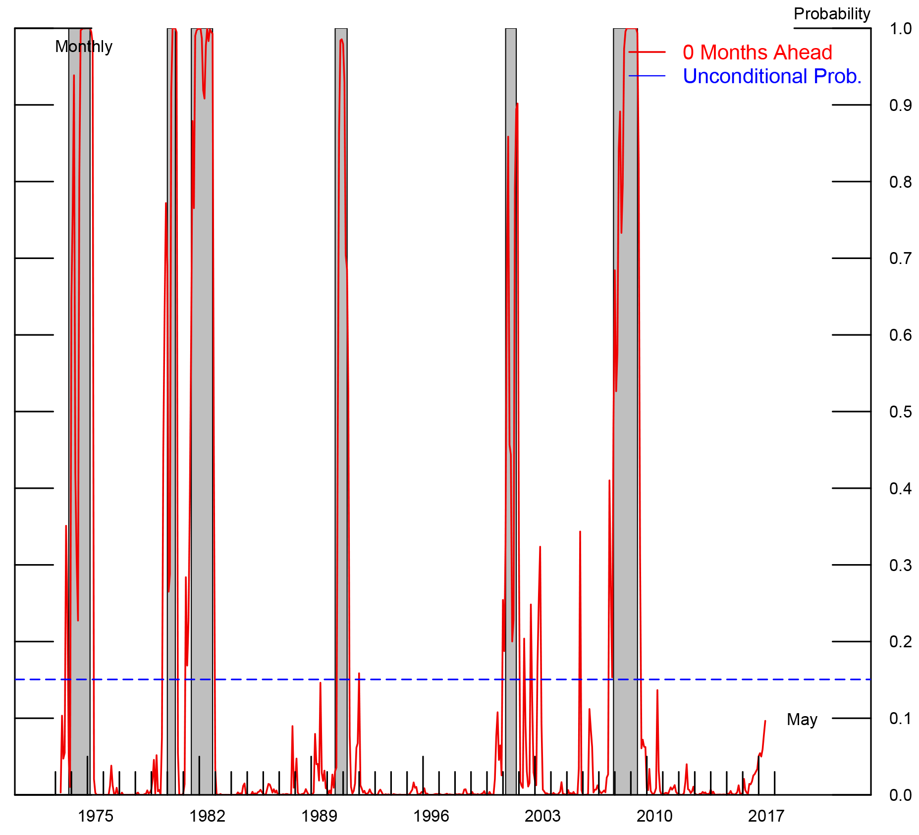
Figure 1 shows how well the BMA model explains historical recessionary periods at two different forecast horizons, 0 and 12 months. A forecast of whether the current month is in recession, known as nowcasting, is shown as the red line in the figure on the left.3 For comparison, the blue dashed line shows the unconditional probability that a given month was declared recession by the NBER, about 15 percent. The estimated recession probabilities fit the historical data quite well, generally rising during recessions which are indicated as the shaded areas.4 The figure on the right asks a more ambitious question: given a particular month's data, what is the probability that 12 months later there will be a recession? Perhaps surprisingly, the fit of this model is also quite good, generally rising alongside the NBER recessions. However, notably the model predicted only a 50 percent chance of recession immediately prior to the Great Recession of 2007-2009, and gave a similar signal in the late 1990's.
 |
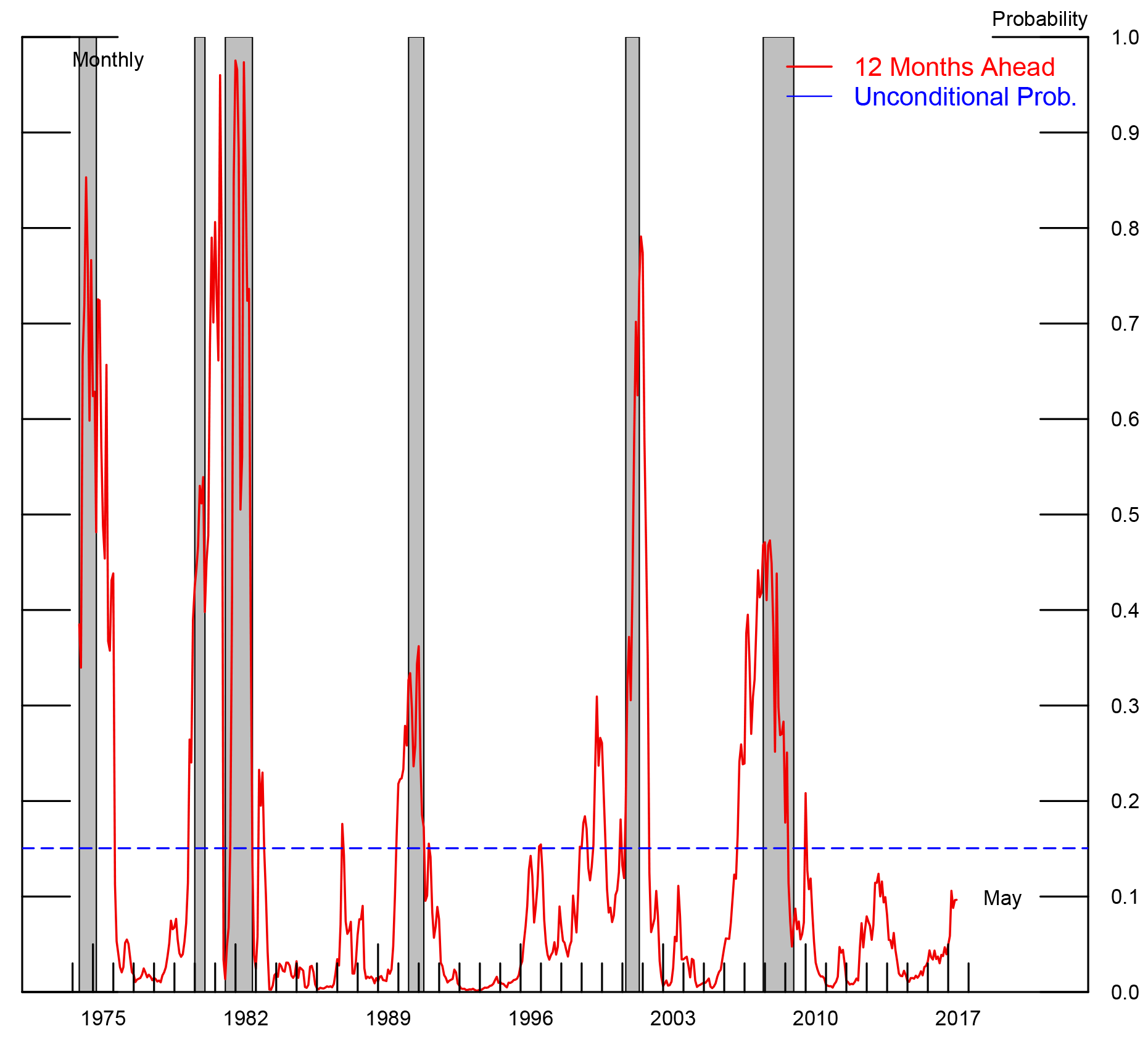 |
Note: Figures show $$ \text{Pr}\ (Y_t \ |\ x_{t-h})$$, so that the date on the x-axis is the forecast that month t was declared recession given information t-h months prior. NBER recession dates shaded.
Which variables matter for signaling recession risks? Table 1 shows variables for which the slope coefficient $$\beta$$ is non-zero at the 90-percent confidence level. The reported coefficients and standard errors are themselves weighted averages from each individual forecasting model, with weights equal to each model's posterior probability (i.e., the $$\hat{w}_i$$'s from equation (2)).5 The importance of each variable can be summarized by its "posterior inclusion probability" -- i.e., the sum of the posterior probabilities of all models that include that particular variable.
As seen in Panel A, the model that evaluates the risk of recession in the current month primarily relies on variables that describe the real economy, such as the number of new jobs created. Interestingly, the model also includes the TED spread, a measure of financial stress that gained prominence during 2007-2009. However, the model that forecasts the probability of recession 12 months hence ignores variables describing real economic activity, relying instead on financial indictors. As seen in Panel B, the model that forecasts recession 12 months from now depends heavily on only two variables: the slope of the Treasury yield curve and the GZ credit spread index, a measure of corporate credit market conditions that is described in detail by Favara, Gilchrist, Lewis, and Suarez (2016).
| Model forecasting the current month | |||
|---|---|---|---|
| Posterior inclusion probability (%) | Coef. | Std. Err. | |
| Panel A: | |||
| Change in payroll employment | 100 | -5.1 | 1 |
| TED spread | 100 | 1.6 | 0.4 |
| Change in initial claims | 99 | -0.2 | 0.1 |
| Panel B: | |||
| Slope of yield curve | 100 | -1.4 | 0.2 |
| GZ index | 100 | 0.8 | 0.4 |
Note: Table shows only indicators with posterior inclusion probability greater than 90 percent.
Evolution of recession risk during 2016
The first half of 2016 has seen mixed economic and financial data. Financial market turmoil at the start of the year has been followed by pockets of disappointing economic news. For example, payroll growth has slowed from its 2015 pace, the decline in commodity prices continues to weigh on particular sectors, and real personal consumption appears to have been tepid in the first quarter of the year. On net, while equity indices remain near their all-time highs, the yield curve has flattened in 2016. Moreover, there have been bouts of financial volatility and periods of high credit spreads. Given this backdrop, we ask: how has the risk of recession, implied by the BMA model, evolved during the course of 2016?
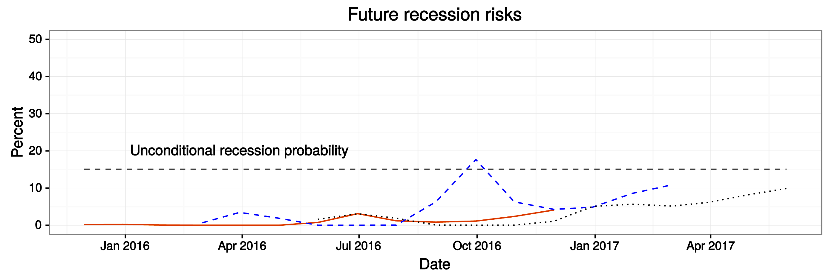
Figure 2 presents a snapshot of the forecasted recession probabilities--ranging from 0 to 12 months ahead--as implied by the model at the three different junctures: November 2015, the orange line; February 2016, the blue dashed line; and May 2016, the black dotted line. As shown, at each of these three junctures the model generally assigned recession probabilities that were below the unconditional probability of the U.S. economy being in recession. A notable excpetion, however, occurred in back February 2016--at that point in time, the model assigned a 17.3 percent probabilitity that October 2016 would be a recession. This spike in recession risk was driven by a deterioration in financial market conditions during February. Since then, financial markets have recovered and the model-implied probabilities of recession have correspondingly declined. In May, prior to the Brexit vote, the model assigned approximately a 10 percent chance that the economy would be in recession 12 months hence.
An important caveat: Forecasting accuracy out-of-sample
While the BMA models were designed to fit the historical pattern of U.S. recessions, an additional issue is how well they perform out-of-sample. A natural question to ask, therefore, is how strong a signal might the BMA methodology have sent ahead of the 2001 and 2008 recessions? To shed light on this issue, we perform a pseudo out-of-sample forecasting exercise by only using data ending prior to the onset of each of these recessions to assess how well the model anticipated the subsequent downturn.6
As shown in Table 2, in September 2001, six months prior to the 2001 recession, the model forecast a 35 percent probability that the U.S. economy would be in recession 12 months from that point in time, well above the unconditional average. The results also indicate that by December, three months ahead of the NBER-dated recession, the model would have sent a fairly strong signal of the impending downturn.
| Forecast made using data through: | ||
|---|---|---|
| Sep-00 | Dec-00 | |
| Current-month | 6 | 4 |
| Three-months hence | 28 | 67 |
| Six months hence | 32 | 57 |
| Twelve months hence | 35 | 39 |
Note: NBER peak dated March, 2001; NBER trough is November, 2001.
Similarly, using data through June 2007, the model forecast a 25 percent probability that the U.S. economy would be in recession 12 months from that point in time. Three months later, with data through September 2007, the model forecast of a recession 12 months had risen to 40 percent.
It is important to bear in mind that most forecasting models do not send very strong signals of recession far ahead of time. To that extent, the fact that BMA sent somewhat elevated readings ahead of prior recessions is reassuring. On the other hand, the BMA recession probabilities ahead of both the 2001 and 2008 recessions were not extraordinarily high, which underscores an important limitation of this exercise, and of forecasting in general.7
| Forecast made using data through: | ||
|---|---|---|
| Jun-07 | Sep-07 | |
| Current-month | 15 | 22 |
| Three-months hence | 26 | 22 |
| Six months hence | 26 | 41 |
| Twelve months hence | 25 | 41 |
Note: NBER peak dated December, 2007; NBER trough is June, 2009.
| Variable | Definition/notes | Transformation |
|---|---|---|
| Financial Variables | ||
| Slope of yield curve | 10-year Treasury less 3-month yield | |
| Curvature of yield curve | 2 x 2-year minus 3-month and 10-year | |
| GZ index | Gilchrist and Zakrajsek (AER, 2012) | |
| TED spread | 3-month ED less 3-month Treasury yield | |
| BBB corporate spread | BBB less 10-year Treasury yield | |
| S 500, 1-month return | 1-month log diff. | |
| S 500, 3-month return | 3-month log diff. | |
| Trade-weighted dollar | 3-month log diff. | |
| VIX | CBOE and extended following Bloom | |
| Macroeconomic Indicators | ||
| Real personal consumption expend. | 3-month log diff. | |
| Real disposable personal income | 3-month log diff. | |
| Industrial production | 3-month log diff. | |
| Housing permits | 3-month log diff. | |
| Nonfarm payroll employment | 3-month log diff. | |
| Initial claims | 4-week moving average | 3-month log diff. |
| Weekly hours, manufacturing | 3-month log diff. | |
| Purchasing managers index | 3-month log diff. | |
Note: Treasury yields from Gurkaynak, Swanson and Wright (2006).
References
Berge, T.J. (2015) "Predicting Recessions with Leading Indicators: Model Averaging and Selection over the Business Cycle," Journal of Forecasting 34(6): 455-471.
Bloom, N. (2009) "The impact of uncertainty shocks," Econometrica 77(3): 623-685.
Blue Chip Financial Forecasts, should be cited as follows: Wolters Klewer. Blue Chip Financial Forecasts. https://lrus.wolterskluwer.com/product-family/blue-chip
Chauvet, M. and J. Piger (2008) "A comparison of the real-time performance of business cycle dating methods," Journal of Business and Economic Statistics 26: 42-49.
Favara, G., S. Gilchrist, K.F. Lewis, E. Zakrajek (2016) "Recession Risk and the Excess Bond Premium," FEDS Notes, April 8.
Gilchrist, S., and E. Zakrajek (2012), "Credit Spreads and the Business Cycle Fluctuations," American Economic Review 102(4): 1692-1720.
Gurkaynak, R., B. Sack and J.H. Wright (2006) "The U.S. Treasury Yield Curve: 1961 to the Present," FEDS Working Paper Series 2006-28.
Hamilton J.D. (2011) "Calling recessions in real time," International Journal of Forecasting 27(4): 1006-1026.
Raftery, A.E. (1995) "Bayesian Model Selection in Social Research," Sociological Methodology 25: 111-163.
1. See the appendix for a complete list of indicators included in our data set. Our dataset begins in January 1973 and ends in May 2016. Some macroeconomic indicators are released with a lag, so that values of very recent months are unavailable at the time of writing. For these indicators, we replace missing values with consensus Blue Chip forecasts and Bloomberg sureys. Return to text
2. Specifically, given our 17 covariates, there are 217--more than 130,000--different potential recession models. We use the method of Raftery (1995) to perform BMA, which approximates the posterior likelihood of each model with a maximum likelihood estimate of it's Bayesian Information Criterion. For further details, see Berge (2015). Return to text
3. Note that nowcasts are not a purely academic exercise, because the NBER dates recessions well after the fact, typically 12 to 18 months after a given recession event. Return to text
4. A more formal evaluation of the model, including an out-of-sample evaluation, is provided in Berge (2015). Return to text
5. For models that do not include a particular variable, BMA sets the coefficient to zero in these cases. Return to text
6. Importantly, owing to data constraints, we use current-vintage data for this exercise. Any judgement on the model's success based on forecasts using revised data should be viewed as an upper-bound on the model capability. Return to text
7. See, for example, Chauvet and Piger (2008), Hamilton (2011), and Berge (2015) for discussions of the real-time performance of several different classes of recession models. Return to text
Please cite as:
Berge, Travis, Nitish Sinha, and Michael Smolyansky (2016). "Which market indicators best forecast recessions?," FEDS Notes. Washington: Board of Governors of the Federal Reserve System, August 2, 2016, http://dx.doi.org/10.17016/2380-7172.1805.
Disclaimer: FEDS Notes are articles in which Board economists offer their own views and present analysis on a range of topics in economics and finance. These articles are shorter and less technically oriented than FEDS Working Papers.
