FEDS Notes
February 17, 2026
Assessing Bank Resilience to a Funding Shock
Faith Achugamonu, Tim Schmidt-Eisenlohr, and Matthew P. Seay1
Introduction
Deposits are the largest source of funding for U.S. banks, representing approximately two-thirds of liabilities. Deposits also remain key to bank profitability, as they typically function as a stable source of long-term funding at a cost well-below interest earned on bank assets. However, a sizable fraction of bank deposits are uninsured, and these deposits can pose additional risks, as demonstrated by the failure of Silicon Valley Bank (SVB) in March of 2023. Following SVB's collapse, a subset of banks experienced growing deposit outflows and were forced to replace those deposits with costlier wholesale funding sources to stabilize their operations (Cipriani et al., 2024; Glancy et al., 2024). In addition, deposit rates began to rise across the banking sector. These factors — deposit outflows and higher funding costs —weakened profitability and intensified concerns about the long-term viability of certain banks.
In this Note, we ask whether a hypothetical system-wide funding shock would significantly impact bank profitability and bank capital ratios. To address this question, we project bank profits and capital using the Forward-Looking Analysis of Risk Events (FLARE) stress testing model.2 We extend the model to incorporate a shock to banks' uninsured deposit funding. In the model, banks with low market-adjusted capital ratios – capital ratios after accounting for changes in the fair values of loans and securities – face higher funding costs on their uninsured deposits.3 This increase in funding costs represents the additional expenses banks incur either by paying higher deposit rates to retain their deposit base or by securing funding from alternative, more expensive sources.4
The effects of this funding shock are illustrated for both the stagflation scenario with severe funding stress from the Board's 2024 exploratory analysis as well as the severely adverse scenario from the Board's 2024 supervisory stress test.5 In the stagflation scenario, adding the funding shock reduces both profitability and capital ratios. This is the case because elevated inflation leads to higher interest rates, which worsens the impact of funding shock for two reasons. First, higher yields reduce banks' market-adjusted capital ratios, causing more banks to be subject to the funding shock. Second, conditional on being hit by the funding shock, higher yields in the stagflation scenario cause a larger repricing effect, because uninsured deposits are repriced to the 3-month Treasury yield plus a 50 bps spread. In contrast, in the severely adverse scenario, adding the funding shock produces minimal effects. This difference arises because during a severe recession without elevated inflation, the Federal Funds rate rapidly declines to zero, substantially reducing both fair value losses on assets and overall funding costs. These contrasting responses highlight how the interest rate environment fundamentally determines how much the funding shock weighs on bank performance.
FLARE Model Overview
FLARE is a top-down, bank-level stress testing model that projects the banking system's pre-provision net revenues (PPNR), loan losses, and capital using public financial statement data and macroeconomic variables.6,7 These macroeconomic variables represent a subset of the 16 domestic variables used in the annual stress test exercise scenarios. Components of PPNR and losses by loan type are individually estimated using regression models that incorporate autoregressive (AR) terms, financial market indicators, macroeconomic variables, and bank-specific control variables. Our estimation sample spans from 1997 to 2024.8 Based on the estimated sensitivities, the model forecasts each bank's income, expenses, loan losses, and resulting capital changes.
Common Equity Tier 1 (CET1) capital is a key measure of financial solvency monitored by regulators. In FLARE, CET1 ratio projections use actual CET1 at the jump-off period, add PPNR, and then subtract loan loss provisions, changes in accumulated other comprehensive income, taxes, and capital payouts.9 To avoid an unrealistic accumulation of capital, it is assumed that banks target CET1 ratios equal to the 4-quarter average of their CET1 ratios at jump-off. Any earnings that would cause a bank's capital ratio to exceed the target level are distributed to shareholders. Otherwise, dividend distributions follow an autoregressive (AR) process and gradually converge toward a long-term payout rate.
Standard measures of regulatory capital, such as CET1, do not fully account for interest rate risk on most securities and loans. Interest rate risk on bank assets primarily stems from their long-term fixed-rate assets, including mortgage loans, government debt, and mortgage-backed securities. The value of these long-term assets declines as long-term yields rise. These unrealized losses can be substantial during a sharp, upward shift in long-term yields, as witnessed when 10-year yields increased about 2.3 percentage points from 2021 through 2022.
To account for these unrealized losses, the FLARE model is augmented with a measure of mark-to-market capital called market-adjusted CET1 (MACET1). MACET1 ratios are calculated by deducting the fair value losses on all securities and loans from the numerator of the CET1 ratios.10,11 MACET1 ratios, in combination with the share of uninsured deposits, represent the key vulnerabilities underlying the funding shock, as discussed in the next section.
Funding Shock Modeling
Banks with weaker fundamentals are more likely to experience funding pressure: they may face larger costs to retain their depositors should stress emerge in the banking system. To incorporate these risks, the funding shock is modeled such that less capitalized banks (those with lower MACET1 ratios) and banks with more reliance on uninsured deposits suffer larger funding cost increases.
We assume a fixed balance sheet and model the funding shock as a repricing of uninsured deposits. That is, a fraction of uninsured deposits gets repriced to a higher rate, which is given by the 3-month Treasury yield plus a spread rate. In reality, at least two things could happen. First, banks could raise deposit rates to help keep deposits in the bank. Second, banks may be unable to retain some portion of their deposit base regardless of rates offered to depositors and may turn to external borrowings to help stabilize their operations. For tractability and to fit with the fixed-balance-sheet assumption, the funding shock only explicitly models the first channel. However, given a sufficiently high repricing rate, the model should capture the quantitative effect of both channels. The funding shock has several characteristics as discussed below.
Which banks are affected?
The model assumes that all banks below a given capital ratio threshold are affected by the funding shock. In the analysis that follows, the funding shock is applied to all banks with MACET1 ratios of 7 percent or less. As of 2024:Q4, the jump-off period in our analysis, about one-fifth of banks had MACET1 ratios less than or equal to 7 percent and are therefore impacted by the funding shock in the first quarter of the scenario.12 This is a conservative assumption, intended to help demonstrate functionality of the funding shock under the assumption of a broad-based financial stress.
What is affected?
The analysis focuses on the repricing of uninsured deposits for two reasons. First, uninsured depositors have stronger incentives than other depositors to withdraw funding in the presence of risk.13 Second, while most banks pay deposit rates well-below market rates, other types of wholesale funding have costs close to or above the Fed Funds rate. Thus, a funding shock applied to more costly funding sources will have a smaller, effect on bank profitability and capital.14
Denote the fraction of the funding that gets repriced as $$\alpha_i$$. This fraction is specified in a flexible way and can vary based on the distance from the capital ratio threshold. $$\alpha_i$$ is given by the following expression
$$$$ \alpha_i = \begin{cases} 0, & \text{if } \mathrm{MACET1}_i \ge \mathrm{CUT}^{up} \\ S^{l} + (S^{h} - S^{l}) \left(\dfrac{\mathrm{CUT}^{up} - \mathrm{MACET1}_i} {\mathrm{CUT}^{up} - \mathrm{CUT}^{low}}\right)^x & \text{if } \mathrm{CUT}^{low} < \mathrm{MACET1}_i < \mathrm{CUT}^{up} \\ S^{h} & \text{if } \mathrm{MACET1}_i \le \mathrm{CUT}^{low}, \end{cases} \ (1)$$$$
where $$S^{h}$$ is the maximum share of funding that gets repriced for affected banks; $$ S^{l}$$ is the minimum share of funding that gets repriced for affected banks; $${CUT}^{up}$$ is the threshold MACET1 ratio below which banks are affected by the funding shock; $${CUT}^{low}$$ is the threshold MACET1 ratio below which banks are affected by the maximum funding shock, where a share $$S^{h}$$ of uninsured deposits gets repriced.15
How are costs affected?
The repricing rate under the funding shock is another key variable. That is, the rate which banks pay instead of the one they are currently paying on their affected uninsured deposits. The quantification presented below assumes a repricing rate given by the 3-month Treasury Yield plus a 50 basis points spread.16 These considerations are captured in equation (2) below.
$$$$ IE_{it} = \begin{cases} \widehat{IE}_{it} & \text{if } \mathrm{MACET1}_i \ge \mathrm{CUT}^{up} \\ \left(1 - \alpha_i UD_i\right)\widehat{IE}_{it} + \alpha_i UD_i RR_t & \text{if } \mathrm{MACET1}_i < \mathrm{CUT}^{up}, \end{cases} \ (2) $$$$
where $$\widehat{IE}_{it}$$ is the average interest expense rate in the absence of the funding shock for bank $$i$$ in period $$t$$; $$UD_i$$ is the share of uninsured deposit in total funding of bank $$i$$; and $$RR_t$$ is the repricing rate for repricing in period $$t$$; and as described above, $$\alpha_i$$ is the fraction of bank $$i$$'s funding that gets repriced.
Figure 1 illustrates how varying parameters in the model change the impact of the funding shock on bank funding costs across banks with different levels of MACET1 ratios. Panel (a) illustrates changes in the funding costs when shape parameter $$x$$ in equation (1) is varied. When $$x$$ = 0, the cost adjustment is the same for all banks below the upper threshold $${CUT}^{up}$$. For $$x$$ = 1, the costs increase linearly as the capital ratio falls up to the point where the MACET1 ratio equals the lower threshold, $${CUT}^{low}$$. From this point on, all banks get a maximum share of funds $$S^{h}$$ repriced. Panel (b) shows funding costs for different levels of $$S^{h}$$ (the maximum share of funds that get repriced). The higher this share, the larger the impact on funding costs. In Panel (c), funding costs are shown for different upper thresholds $${CUT}^{up}$$. The higher this threshold is, the more banks are affected by the funding shock.
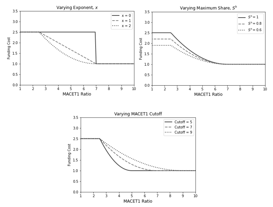
Notes: Parameter values for illustration unless indicated otherwise: $$CUT^{up} = 7; CUT^{low} = 2.5; x=1; S^h = 1; S^l = 0; RR=$$ 3-month Treasury yield +50 bps; 3-month Treasury yield = 4.25 percent; $$UI$$ = 0.4.
Funding Shock Illustration
Next, we illustrate the effects of the funding shock in FLARE in the stagflation scenario with severe funding stress from the Board's 2024 exploratory analysis. We also briefly discuss how effects of the funding shock differ in the severely adverse scenario from the Board's 2024 annual stress test.17 Our jump-off period is 2024:Q4, and we project bank profitability and capital through 2027:Q1.
We apply the shock to any bank that falls below a MACET1 ratio of 7 percent and assume uninsured deposits reprice towards the 3-month Treasury yield plus 50 basis points. The strength of the effect is assumed to increase linearly with distance from the upper cutoff, that is, we set shape parameter x to one. Uninsured deposits are fully repriced for banks with a MACET1 ratio at or below 2.5 percent of risk-weighted assets.
How do the macro scenarios considered in this exercise differ?
While our main analysis focuses on the severe stagflation scenario, in the following, we also describe the severely adverse scenario, which generally mimics dynamics observed during the Global Financial Crisis. Both scenarios have similar paths for real variables, with the unemployment rate climbing to 10 percent in each and remaining elevated. The key difference between the two scenarios is the path for inflation, which leads to different paths for interest rates. In the severely adverse scenario, the Fed cuts rates to support the economy as real activity declines and the 10-year Treasury yield dips to about 1 percent (figure 2, right panel). By contrast, in the stagflation scenario, the Fed raises rates despite the recession to combat elevated inflation, causing the 10-year yield to increase to approximately 5 percent before declining slightly (figure 2, left panel).
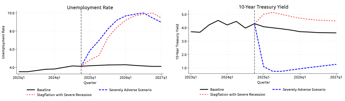
Source: Federal Reserve, Annual Stress Test Scenarios, (https://www.federalreserve.gov/supervisionreg/dfa-stress-tests-2024.htm)
How does the funding shock impact banking system profitability?
The impact of the funding shock is captured directly through net interest margins (NIM), which are the difference between interest earned on loans and securities and interest paid on deposits, debt, and other borrowings divided by interest-earning assets. The left panel of figure 3 shows the weighted average banking system NIMs in the stagflation scenarios with and without funding shock and NIMs in the more benign baseline scenario.
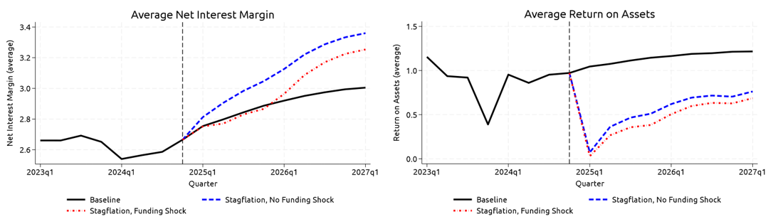
Source: FR Y-9C, Call Reports, Federal Reserve, Annual Stress Test Scenarios. (https://www.federalreserve.gov/supervisionreg/dfa-stress-tests-2024.htm)
NIMs increase materially in the stagflation scenario without funding shock, as higher yields lift interest earnings on variable rate loans and securities, while funding costs increase by less because banks only partially pass through rate increases to deposit rates. In contrast, banking system NIMs are slightly below baseline levels for about a year in the stagflation scenario with funding shock, despite a more favorable interest rate environment.18 This is because a subset of banks is hit by the funding shock. The funding shock causes them to pay higher rates on their uninsured deposits, which leads to a compression of banking system return on assets – or total net income divided by assets – as shown in the right panel of figure 3.19 Of note, the higher yields in the stagflation scenario worsen the funding shock in two ways: they directly increase the repricing rate and weigh on market-adjusted capital, pushing more banks below the funding shock MACET1 threshold.
How does the funding shock impact banking system capital?
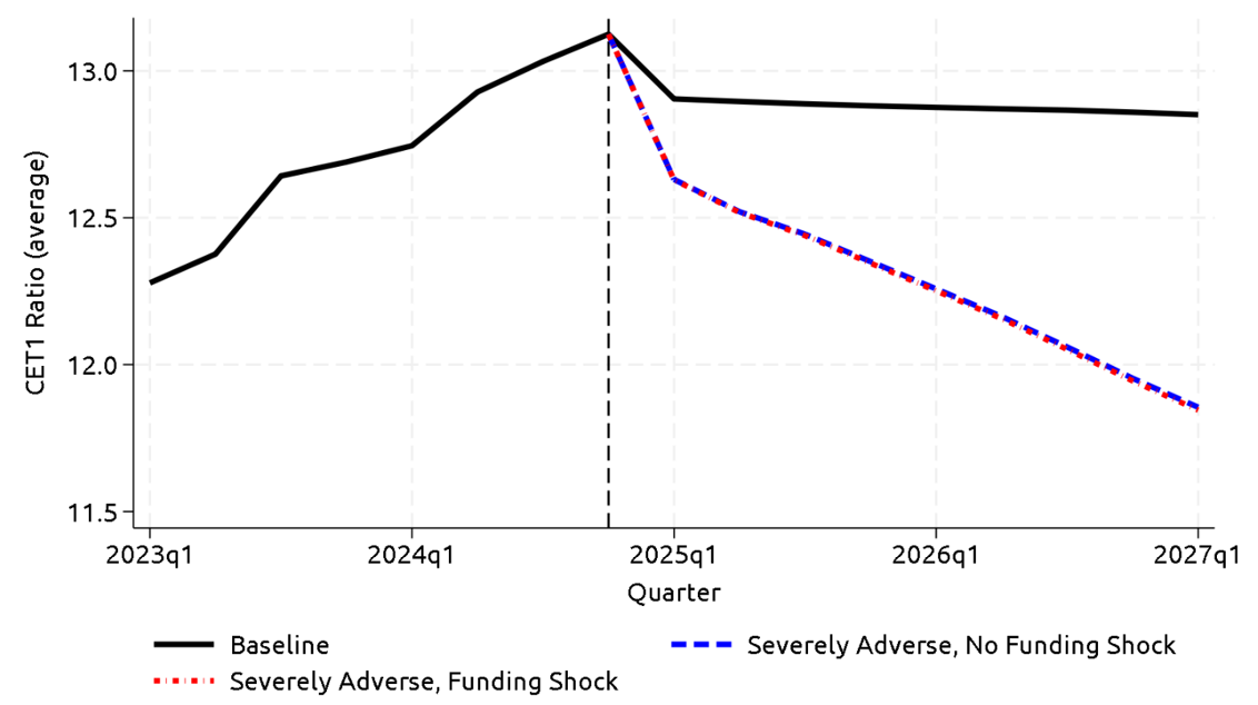
Figure 4 shows banking system common equity tier 1 (CET1) ratios – a regulatory measure of bank solvency – in the stagflation scenarios with and without funding shock and in the baseline scenario (also provided in the Board's annual stress test). The severe real conditions in the stagflation scenario cause material declines in capital relative to the more benign baseline scenario. The funding shock leads to additional declines in aggregate banking system capital. The additional declines are relatively small, however, because most banks remain profitable.
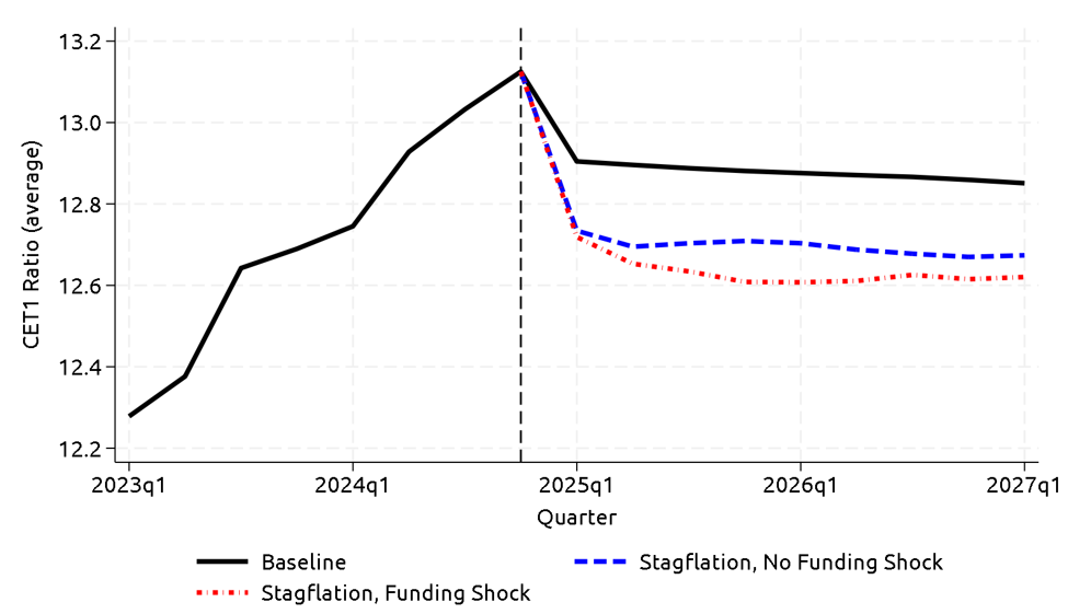
Note: We assume banks target capital levels equal to the 4-quarter average of their CET1 ratios. CET1 ratios decline across all scenarios during the first projection period as any capital in excess of the firm's target CET1 ratio is paid out at that time.
Source: FR Y-9C, Call Reports, Federal Reserve, Annual Stress Test Scenarios. (https://www.federalreserve.gov/supervisionreg/dfa-stress-tests-2024.htm)
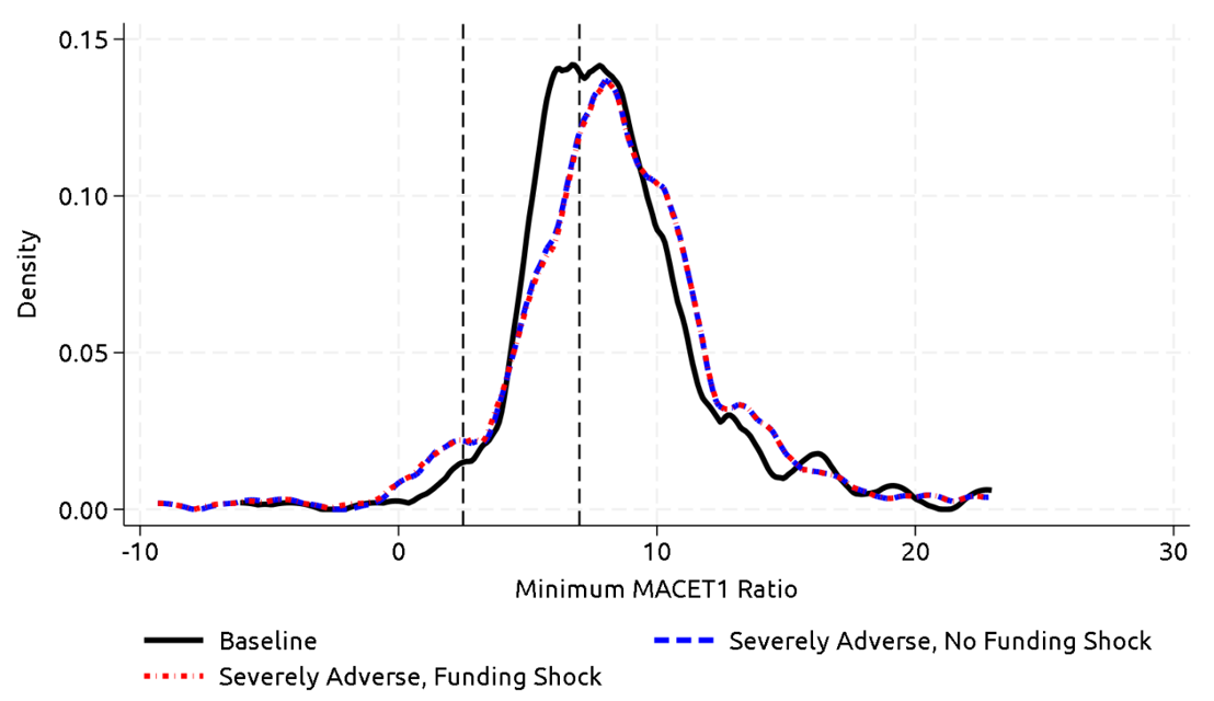
Increases in long-term yields reduce the fair value of banks' long-term fixed rate loans and securities. As discussed before, these changes are accounted for in MACET1 ratios, a non-regulatory measure of capital. Figure 5 shows the distribution of post-stress minimum MACET1 ratios for each scenario.20 In the stagflation scenario without funding stress, banks with larger shares of long-term fixed rate assets observe sizable declines in their MACET1 ratios, as demonstrated by the leftward shift of the distribution shown by the blue line. Post-stress minimums worsen further when the funding shock is applied, as evidenced by an additional leftward shift and an increase in mass of firms with MACET1 ratios below zero.
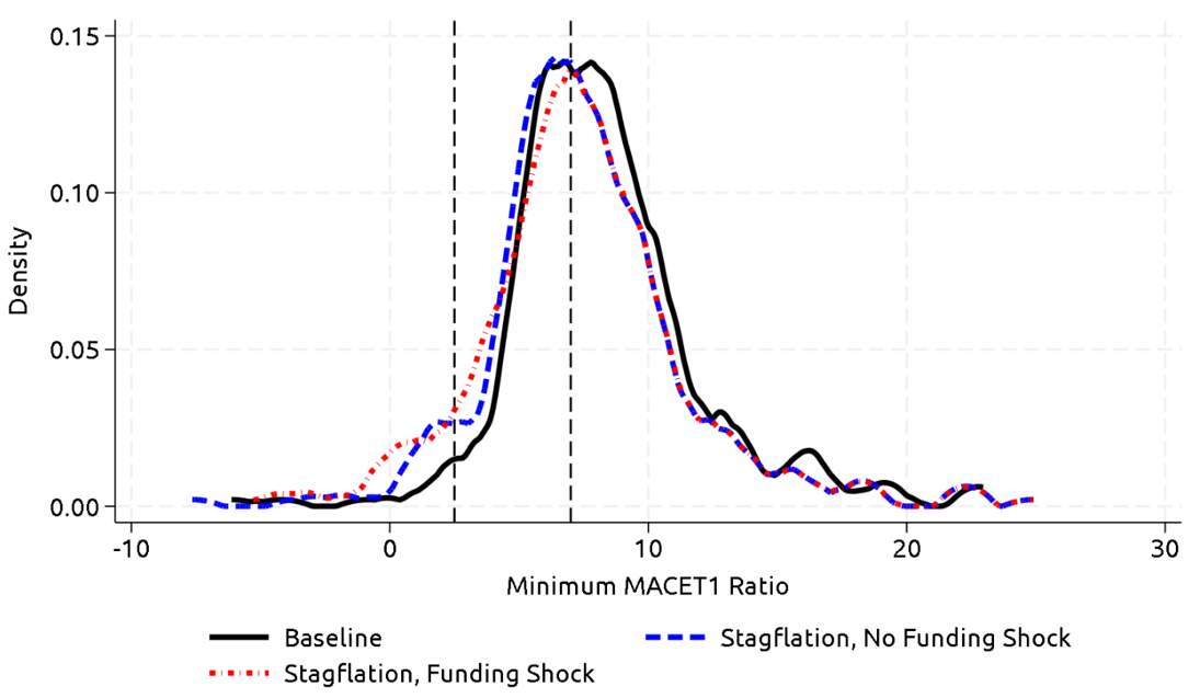
Note: The right-most dashed vertical line denotes the threshold at which uninsured deposits start to reprice in the funding shock. The left-most dashed vertical lines denote the threshold at which a bank's entire uninsured deposit base reprices to the 3-month Treasury yield plus the 50 basis points spread.
Source: FR Y-9C, Call Reports, S&P Capital IQ Pro, FR Y-14Q, Schedule B, FR Y-14Q, Schedule G, Federal Reserve, Annual Stress Test Scenarios. (https://www.federalreserve.gov/supervisionreg/dfa-stress-tests-2024.htm)
How does increasing the repricing rate impact banking system solvency?
In this section we study how the effect of the funding shock on banking system capital ratios varies with the repricing rate. In this illustration, we hold all other funding shock parameters fixed.
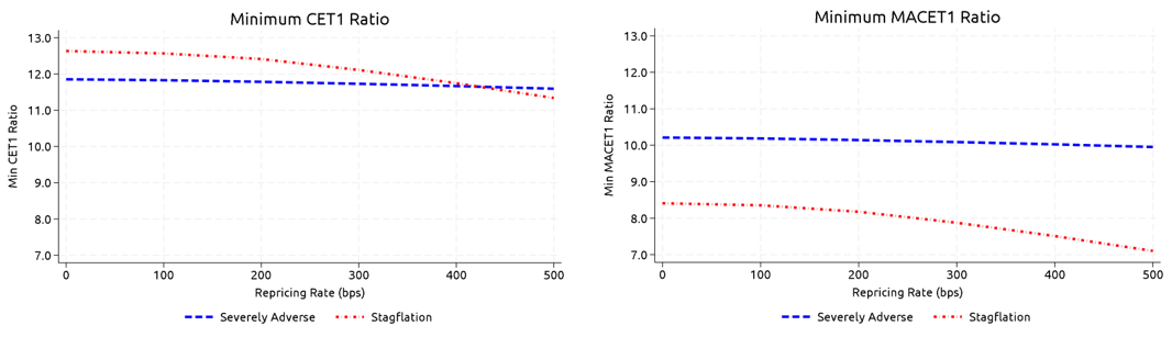
Figure 6 shows that increasing the repricing rate on uninsured deposits significantly decreases the post-stress minimum banking system CET1 ratios (left panel) and MACET1 ratios (right panel) in the stagflation scenario by more than 1 percentage point but has minimal effects in the severely adverse scenario. This is the case for two reasons. First, lower interest rates boost the fair value of bank assets in the severely adverse scenario, which increases market-adjusted capital and limits the number of banks that face funding shocks. Second, the level of 3-month Treasury yields remains significantly lower in the severely adverse scenario and thus has smaller effects on bank funding costs.
Figure 6. Impacts of Varying the Repricing Rate21
Source: FR Y-9C, Call Reports, S&P Capital IQ Pro, FR Y-14Q, Schedule B, FR Y-14Q, Schedule G, Federal Reserve, Annual Stress Test Scenarios. (https://www.federalreserve.gov/supervisionreg/dfa-stress-tests-2024.htm)
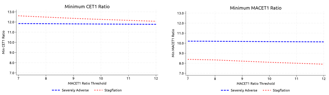
Next, we conduct a similar exercise and change the MACET1 ratio threshold at which we begin to reprice uninsured deposits. As the threshold is raised, an increasing number of banks are exposed to higher uninsured deposit costs. In the stagflation scenario, raising MACET1 ratio threshold from 7 percent to 12 percent causes an additional decline of about 0.5 percentage points in banking system CET1 ratios (figure 7, left panel) and MACET1 ratios (figure 7, right panel).
Source: FR Y-9C, Call Reports, S&P Capital IQ Pro, FR Y-14Q, Schedule B, FR Y-14Q, Schedule G, Federal Reserve, Annual Stress Test Scenarios.
Conclusion
In this note we introduced an extension to the FLARE stress testing model that allows us to analyze some risks associated with funding shocks. We find that funding shock risks are most pronounced in an environment with high interest rates. However, even in the stagflation scenario considered here, the bank funding shock only has a moderate effect on aggregate banking system regulatory capital ratios. In part, the moderate impact is due to the recent reduction in runnable funding and asset duration in the banking system since the SVB failure. The shock is most severe for banks with high asset duration and significant reliance on runnable funding, but there are a very limited number of banks facing both vulnerabilities.
One caveat of our analysis is that the funding shock only hits deposit costs. In reality, a bank with large deposit outflows or a bank facing significant deposit repricing and profitability pressures may also see other parts of its business affected. For example, counter-parties may become worried about the viability of the bank and pull deposits faster than what our exercise assumes. In addition, publicly-traded banks might experience substantial pressures from investors, which could lead to large equity price declines and additional depositor flight.
A benefit of FLARE is that its modular structure provides flexibility to consider a variety of evolving risks. It is unlikely that the next set of bank failures will resemble the last. And thus, FLARE will continue to evolve and to test alternative scenarios to better understand the relationship between the resiliency of the banking system and the macroeconomy.
References
Armantier, Olivier, Marco Cipriani, and Asani Sarkar (2024), "Discount window stigma after the global financial crisis." FRB of New York Staff Report.
Cipriani, Marco, Thomas M Eisenbach, and Anna Kovner (2024), "Tracing bank runs in real time." FRB of New York Staff Report.
Correia, Sergio, Matthew P Seay, and Cindy M Vojtech (2022), "Updated primer on the forward-looking analysis of risk events (flare) model: A top-down stress test model." FEDS Working Paper.
Drechsler, Itamar, Alexi Savov, Philipp Schnabl, and Olivier Wang (2023), "Deposit franchise runs." National Bureau of Economic Research.
Glancy, David, Felicia Ionescu, Elizabeth Klee, Antonis Kotidis, Michael Siemer, and Andrei Zlate (2024), "The 2023 banking turmoil and the bank term funding program."
Hirtle, Beverly, Anna Kovner, James Vickery, and Meru Bhanot (2016), "Assessing financial stability: The capital and loss assessment under stress scenarios (class) model." Journal of Banking & Finance, 69, S35–S55.
Appendix
What do results look like under the severely adverse scenario?
In the severely adverse scenario, inflation is subdued, and the 3-month Treasury yield drops to the zero lower bound while the 10-year rate declines markedly. The lower yields reduce the effect of the funding shock in two ways: first, lower long-term yields boost MACET1 ratios, leaving fewer banks below the funding shock cutoff. Second, when short rates are low, the repricing rate (3-month Treasury yield plus the 50 basis points spread) mildly increases funding costs at banks hit by the funding shock. These considerations are reflected in figures A1 and A2 that show the banking system CET1 ratio and the MACET1 distributions under the severely adverse scenario. As expected, the funding shock does not materially affect the aggregate CET1 level or the distribution of MACET1 ratios.
Source: FR Y-9C, Call Reports, Federal Reserve, Annual Stress Test Scenarios. (https://www.federalreserve.gov/supervisionreg/dfa-stress-tests-2024.htm)
Source: FR Y-9C, Call Reports, S&P Capital IQ Pro, FR Y-14Q, Schedule B, FR Y-14Q, Schedule G, Federal Reserve, Annual Stress Test Scenarios. (https://www.federalreserve.gov/supervisionreg/dfa-stress-tests-2024.htm)
1. Achugamonu, Schmidt-Eisenlohr, and Seay are staff in the Division of Financial Stability at the Federal Reserve Board. The views in this Note are solely those of the authors and should not be interpreted as reflecting the views of the Board of Governors of the Federal Reserve System. We thank Sergio Corriea for his substantial contributions to the development of the stress testing model used in this analysis. We thank William Bassett, Jose Berrospide, Skander Van den Heuvel, and Cindy Vojtech for their helpful comments. Return to text
2. For a primer on FLARE, see Correia et al. (2022). Return to text
3. The analysis abstracts from the possibility that outflows from weaker banks may stay in the banking system and flow toward better capitalized banks. Return to text
4. Banks unable to secure funding or maintain their deposit base by offering higher deposit rates may be forced to shrink their balance sheets. However, in this exercise we assume a fixed balance sheet throughout the simulation. Consequently, the funding shock in our model operates solely through adjustments to interest expenses rather than changes in either aggregate quantities or in the composition of liabilities. Return to text
5. Details on the Board's 2024 stress test and exploratory analysis are available here: https://www.federalreserve.gov/supervisionreg/dfa-stress-tests-2024.htm Importantly, these scenarios do not represent forecasts and the interest rate paths in the scenarios follow a rule that does not necessarily reflect the actual response by the FOMC if these scenarios materialized. Return to text
6. FLARE is built from the Capital and Loss Assessment under Stress Scenarios (CLASS) model foundation. For more information on the CLASS model see Hirtle et al. (2016). Return to text
7. Top-down models use bank-level data, as opposed to a bottom-up model that would use more granular data such as loan-level and security-level data. Many of the models used to project losses in the annual stress test exercises are bottom-up models. FLARE is constructed using mostly bank-level data from FR Y-9C and Call Reports. FR Y-9C filers include all bank holding companies with at least $3 billion in consolidated assets. Call report filers include commercial banks regardless of asset size. Commercial banks are consolidated to their parent for use in the model. Return to text
8. The COVID-19 pandemic and the sizeable fiscal and monetary policy responses created significant disruptions in the historical relationships between macroeconomic variables and bank performance metrics. To address these concerns in our modeling framework, we applied data smoothing techniques and substituted historical averages for macro variables during the pandemic period. This methodological adjustment prevents pandemic-specific distortions from biasing our model's parameter estimates while preserving the longer time series. Return to text
9. Profits are taxed at 21 percent. Return to text
10. Liabilities are excluded. The fair value of bank liabilities also fluctuates with interest rate movements and can function as a natural hedge against declines in asset fair values. However, as events in 2023 demonstrated, this hedge can be fragile under stress. Return to text
11. Historical securities fair-value losses are sourced from regulatory filings including FR Y-9C and Call Reports. Hypothetical securities losses in scenarios are projected using changes in yields in each scenario, duration data from FR Y-14Q, Schedule B, and the maturity/repricing time distribution of securities from Call Reports. Historical loan fair values are sourced from S&P Capital IQ Pro for publicly traded banks. For all other banks, we estimate historical loan fair values as a function of publicly traded banks' historical loan fair values. Hypothetical loan fair value projections are estimated using changes in yields in each scenario, the maturity/repricing time distribution of loans from Call Reports, and select weighted average life information from FR Y-14Q, Schedule G. Return to text
12. In the model, the funding shock is based on the previous quarter's MACET1 ratio. For example, in 2025:Q1, a bank is affected by the funding shock if its MACET1 ratio in 2024:Q4 is below 7 percent. Return to text
13. See, e.g., Drechsler et al. (2023). Return to text
14. Still, one could imagine alternatives where all deposits get repriced. In addition, other sources of funding, like wholesale funding, could experience cost increases at varying repricing rates. Return to text
15. For all analysis presented in this note, we set $$S^{h}$$ equal to one and $$S^{l}$$ equal to zero. Return to text
16. This assumption is flexible. The repricing rate assumption used in this analysis is in line with estimates provided by Armantier et al. (2024). Return to text
17. Additional results from the severely adverse scenarios are shown in the appendix. Return to text
18. As discussed earlier, the exercise assumes a fixed balance sheet. In reality, stagflation may have real effects that could cause contractions in bank lending volumes which are not reflected in our analysis. Return to text
19. While the funding shock reduces banks' average return on assets modestly, the large drop in return on assets in the stagflation scenario is primarily caused by other scenario features. These include a severe deterioration in asset prices and financial conditions, which is associated with large declines in non-interest income. Return to text
20. For each bank we calculate the minimum MACET1 ratio over the 9-quarter stress test horizon. These minimum MACET1 ratios are then combined in one density distribution. Return to text
21. The two charts illustrate the effect of varying the repricing rate over the 3-month Treasury yield from 0 to 500 basis points. This range of values is meant to illustrate the model mechanics and should not be seen as suggesting that banks would realistically pay a spread of 500 basis points over the 3-month Treasury yield. Return to text
Achugamonu, Faith, Tim Schmidt-Eisenlohr, and Matthew P. Seay (2026). "Assessing Bank Resilience to a Funding Shock," FEDS Notes. Washington: Board of Governors of the Federal Reserve System, February 17, 2026, https://doi.org/10.17016/2380-7172.3987.
Disclaimer: FEDS Notes are articles in which Board staff offer their own views and present analysis on a range of topics in economics and finance. These articles are shorter and less technically oriented than FEDS Working Papers and IFDP papers.