FEDS Notes
September 24, 2025
Homeownership and Housing Equity in the Mid-Twentieth Century
Carola Frydman, Raven Molloy and Austin Palis1
1. Introduction
Housing is an important component of wealth for most American households (Bricker, Moore and Thompson 2019; Kuhn et al., 2020), so studying trends in homeownership can shed light on changes in aggregate household wealth and how it is distributed across families. The aggregate US homeownership rate increased by 20 percentage points from 1940 to 1960, the largest change in American homeownership in the past 100 years. Prior research has attributed this rapid increase to several factors, including an expansion of mortgage credit (Fetter 2013; Chambers, Garriga and Schlagenhauf 2014), increases in household income (Collins and Niemesh 2025), and changes in the age distribution (Fetter 2014). However, little is known about how the increase in homeownership rates during this unique period varied for households with different characteristics.2
The types of families that entered homeownership during the 1940s and 1950s may have long-lasting implications for the distribution of wealth. Prior work has documented that increases in house prices were a key driver of increases in household wealth from 1971 to 2007 (Kuhn et al. 2020). Yet only homeowners benefited from these rising house prices. Given the strong intergenerational persistence of housing wealth (Benetton, Kudlyak and Mondragon 2024; Daysal, Lovenheim and Wasser 2023) and relative stability of homeownership post-1960, it was the types of families that were homeowners by 1960 who were able to benefit from the subsequent house price appreciation. In this analysis, we shed light on this important question by documenting changes in homeownership mid-century by two key family attributes: current annual family income and an estimate of permanent family income that accounts for family characteristics such as education and occupation of the head.
Research on changes in homeownership during the 1940s and 1950s has been hampered by a lack of household-level data. Although the 1940 and 1960 Decennial Census provide some information about the endpoints of this 20-year period, the 1950 Census of Housing microdata were never digitized and the paper records no longer exist.3 In this analysis, we study annual changes in homeownership for the later part of this period—from 1947 to 1960—using family-level data from the Survey of Consumer Finances (SCF). In addition to shedding light on changes in homeownership at a higher frequency than available in the Decennial Census, the SCF provides richer information than the Census, allowing us to examine changes in mortgage use, home equity, and other asset holdings, as well as homeownership.
The SCF was administered annually by the University of Michigan Survey Research Center from 1947 through 1971 and the data are made publicly available through the University of Michigan's Inter-university Consortium for Political and Social Research. The unit of observation in the SCF is a "spending unit," which is defined as a group of related people living in the same dwelling unit who pool their incomes for their major items of expense. We only use data for primary spending units, which are spending units containing the head of the household, because we want our estimates to be comparable to household-level estimates from the Decennial Census. We also drop spending units that report living on a farm to abstract from changes in homeownership resulting from the demographic transition from farms to urban areas. In what follows, we refer to spending units as families. The resulting SCF sample contains about 2,000 families per year on average.
We find that increases in homeownership were concentrated among families with higher annual income and with higher permanent income—i.e., those with heads in white-collar occupations and with more education. Because these families had higher homeownership rates in 1947, the homeownership gap between these families and lower-income families widened materially from 1947 to 1960. We also show that this widening in homeownership rates across the income distribution was partly related to reductions in the affordability of purchasing a home, as house prices rose at least as much as incomes. Moreover, the amount of liquid savings held by lower-income families was generally not large enough for a downpayment on a house during this period, whereas higher-income families tended to have more liquid savings. Changes in mortgage credit access, particularly for veterans, may also have contributed to the trends in homeownership inequality over this period. Higher fertility rates during the Baby Boom and an increase in suburbanization may have also played a role by boosting the demand to live in larger, single-family, and more expensive homes. We conclude by showing that the changes in homeownership rates across the distribution of income led to growing differences in housing wealth across groups during this period.
2. Changes in homeownership over time
Figure 1 shows the aggregate homeownership rate in the SCF and Decennial Census from 1940 to 1960. In the two years when the data sources overlap (1950 and 1960) the homeownership rates are remarkably similar, which gives us confidence to rely on the SCF to examine these changes in more detail.4 Overall, the homeownership rate increased from 41 percent in 1940 to 61 percent in 1960. About 60 percent of this increase took place from 1940 to the start of the SCF sample in 1947, when the aggregate homeownership rate was 53 percent.5 After 1947, homeownership continued on a general upward trend, with perhaps two periods of faster increases from 1949 to 1951 and from 1955 to 1957.
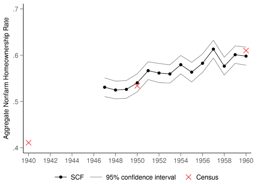
Source: Author calculations from the Survey of Consumer Finances 1947-1960, the 1940 and 1960 Censuses using data from IPUMS (Ruggles et al. 2025), and the 1950 Census of Housing Volume 1, Table 2.
Figure 2 takes an initial look at how the rise in homeownership from 1947 to 1960 was distributed across families by showing the average homeownership rate for each quintile of the distribution of total family income.6 We cannot examine changes in homeownership by total family income between 1940 and 1947 because the 1940 Census only reported labor income, not income from other sources.7 Figure 2 shows that families in the top three quintiles of the total income distribution experienced material increases in homeownership, whereas homeownership was flat for the families in the bottom two quintiles.

Source: Author calculations from the Survey of Consumer Finances 1947-1960 and the 1960 Census using data from IPUMS (Ruggles et al. 2025).
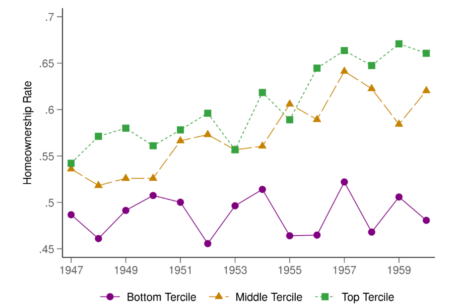
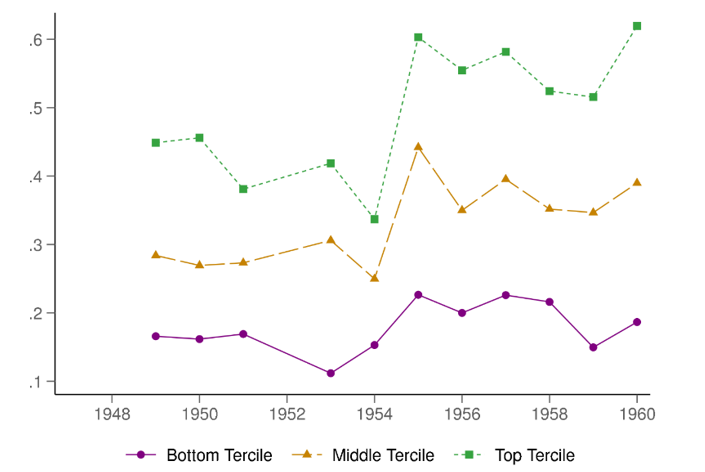
Housing decisions are usually made based on a longer-term assessment of a family's income prospects because moving is costly. Annual income is an imperfect measure of a family's permanent income for several reasons. One reason is the typical lifecycle trajectory of income—i.e., young individuals may have low current incomes but might expect to have high incomes later in life. The housing decisions of people who expect high income growth might be quite different from those of older people who have similarly low incomes. Second, annual income can be volatile (Guvenen et al. 2021). For these reasons, we construct a measure of predicted permanent income of the family by regressing the natural logarithm of total family income on indicators for the head's education, the head's occupation, the head's age, the number of earners in the family, and year.8 We predict income using the coefficients on education, occupation and number of earners, but not age or year. Therefore, this measure of predicted income reflects the likely income of the family given the head's education and occupation and the number of earners in the family—features that should be relatively invariant to the head's current point in the lifecycle and to transitory fluctuations in income. Table 1 summarizes the characteristics of families across the distribution of predicted income. Families in the bottom tercile of predicted income were more likely to have heads without a high school education and in service or laborer occupations. In addition, they were less likely to have multiple earners in the family. Figure 3 shows that families in the top two terciles of predicted income experienced increases in homeownership, whereas those in the bottom tercile did not. Consequently, these results show that it was families with higher permanent income that experienced rising homeownership during this period.
Table 1: Family Characteristics by Tercile of Predicted Income
percent
| Predicted Income Terciles | |||
|---|---|---|---|
| Bottom | Middle | Top | |
| Education of Head | |||
| Less than high school | 83.4 | 26.7 | 2.7 |
| Some high school or diploma | 15.6 | 64.9 | 48.4 |
| More than high school | 1 | 8.4 | 48.9 |
| Occupation of Head | |||
| Self Employed | 0 | 8.8 | 27.3 |
| Salaried Professional | 2 | 9.3 | 33.6 |
| Clerical/Sales | 6.2 | 24.5 | 11.3 |
| Skilled/Semi-skilled | 39.3 | 56.9 | 27.8 |
| Unskilled | 52.5 | 0.5 | 0 |
| Number of Income Earners in Family | |||
| One | 82.3 | 81.6 | 43.9 |
| Two | 15.6 | 16.6 | 52.1 |
| Three or more | 2.1 | 1.8 | 4 |
| Veteran Status of Head | |||
| Non-veteran | 81 | 68.4 | 61.3 |
| Veteran | 19 | 31.6 | 38.7 |
| Race of Head | |||
| White | 80.9 | 94.6 | 96.6 |
| Black | 19.1 | 5.4 | 3.4 |
| Age of Head and Marital Status | |||
| Percent married and younger than 35 | 18.9 | 28.4 | 30.9 |
Note: Veteran status refers to World War II and the Korean War. Income is predicted using the number of earners in the family and the education and occupation of the head.
Source: Author calculations from the Survey of Consumer Finances 1947-1960.
Note: Family income is predicted using the number of earners in the family and the education and occupation of the head.
Source: Author calculations from the Survey of Consumer Finances 1947-1960.
3. Explanations for divergence in homeownership by income group
Why did homeownership increase more for higher-income, white-collar, and more-educated families from 1947 to 1960? Many changes in the US economy during this period likely contributed to the rise in the aggregate homeownership rate. Real incomes were rising and the post-war baby boom likely increased demand to live in single-family homes, which tend to be owner-occupied. In addition, a massive construction boom in the suburbs expanded the supply of owner-occupied homes. Growing availability of affordable cars and an expansion of the US highway system also improved access to these suburban homes. Meanwhile, an expansion of mortgage credit availability may also have improved access to homeownership. In this section, we address each of these factors in turn, focusing on which types of families were likely influenced by each one. We highlight that our analysis does not provide causal estimates of the contributions of any single factor.
A natural place to start is to consider the incomes of the families in each of these groups. Figure 4 shows that the median income in each tercile of predicted income rose by roughly the same amount during this period. But income gains would not necessarily lead to increases in homeownership if house prices were rising too. Figure 4 also shows the 25th percentile of the distribution of house values in the SCF as an estimate of the price of a smaller, lower-quality home that would be the target of a first-time homebuyer. House prices rose by at least as much as median income in each tercile during this period, showing that homes were getting more expensive even as family incomes were rising.
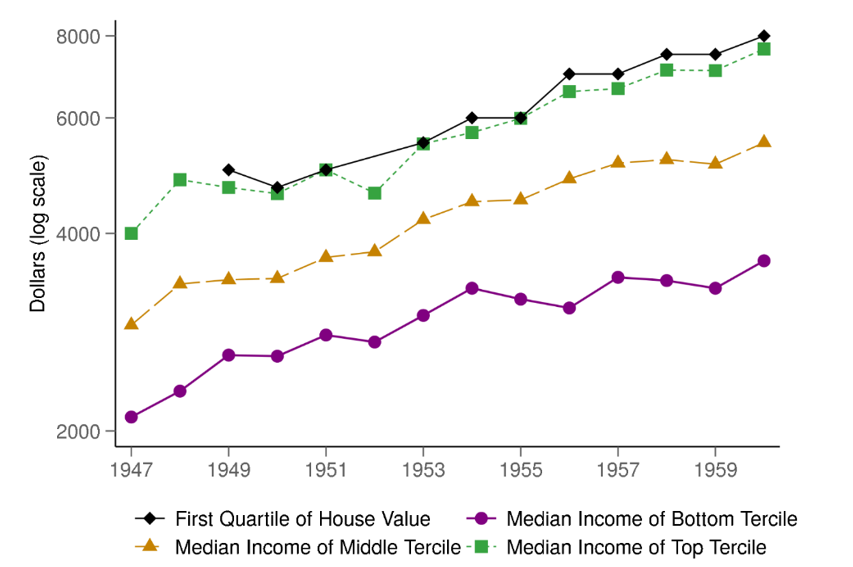
Note: House value is not reported in 1948, 1949 and 1952.
Source: Author calculations from the Survey of Consumer Finances 1947-1960.
Even though incomes were rising for families in all three terciles during this period, one possible reason for the divergence in homeownership rates is that the level of income for families in the bottom tercile just wasn't high enough to allow them to transition into homeownership. To assess the affordability of becoming a homeowner, ideally we would like to compare renter incomes to the income needed to become a first-time homebuyer. It is difficult to calculate this level of income because doing so would require detailed information on mortgage underwriting standards, borrower characteristics and house prices. But we can get a rough sense of this income target by examining the incomes of first-time homebuyers. In 1955, the only year in our sample period when the SCF recorded first-time buyer status, about 3/4 of first-time buyers were age 25-44. As a proxy for the income of first-time homebuyers, Figure 5 shows the distribution of income among families with a head in this age range that purchased a home recently (in the current year or previous year). Figure 5 also shows the distributions of income for renters in the bottom and middle terciles of predicted income. Most of the renters in the bottom tercile had incomes substantially lower than the incomes of (likely) first-time homebuyers, suggesting that their income was too low for them to transition into homeownership. By contrast, there is much more overlap between the distribution of income of middle-tercile renters and the incomes of first-time homebuyers.
Figure 5. Distribution of Income for Renters in the Bottom and Middle Terciles of Predicted Income and First-Time Homebuyers
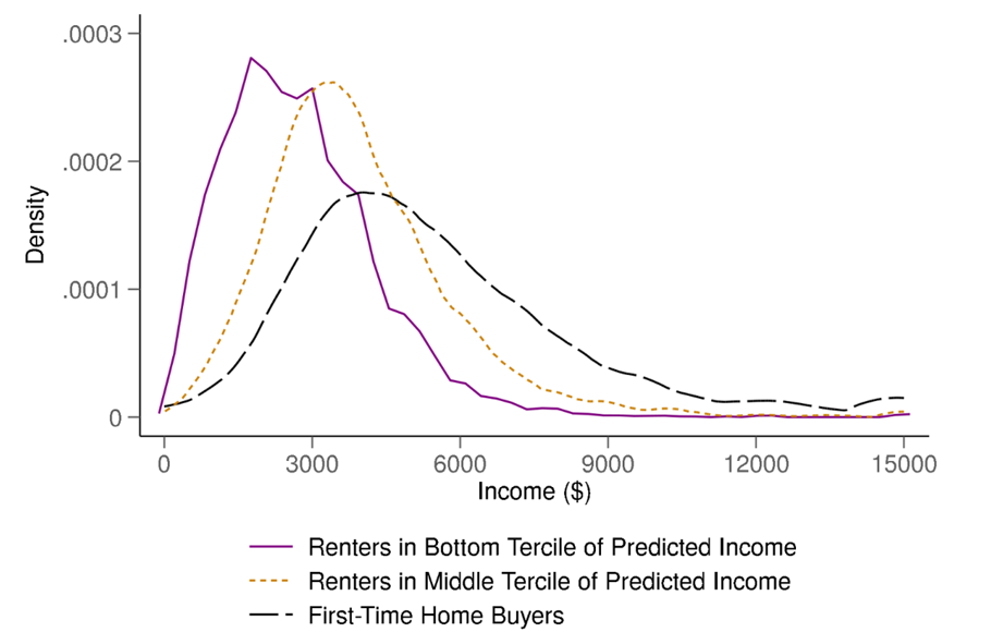
Note: Family income is predicted using the number of earners in the family and the education and occupation of the head. First-time homebuyers are families with a head age 25 to 44 that bought a home in the current or previous year.
Source: Author calculations from the Survey of Consumer Finances 1947-1960.
Another issue related to housing affordability is the need to have enough money to afford a downpayment. As a gauge of whether renter families had sufficient resources to afford a downpayment, we examine their liquid assets relative to the amount needed for a downpayment on an FHA loan. We focus on FHA mortgages because their downpayment requirements tended to be lower than for conventional loans made by savings and loan institutions (Herzog and Earley 1970). Specifically, Federal Housing Administration (FHA) mortgages required a downpayment of at least 20 percent of the value of the home from 1947 to 1954. The Housing Act of 1954 decreased this requirement to as low as 5 percent or as much as 16 percent, depending on loan size (Federal Housing Administration, 21st Annual Report). Regarding the family's financial resources, we use liquid assets, which includes savings accounts, checking accounts and bonds. Of course, liquid assets are not the only source of a downpayment for first-time homebuyers. For example, they might sell illiquid assets like stocks or bonds or receive gifts from family members. That said, the SCF asked recent homebuyers the source of their downpayment in 1949, and liquid assets were the reported source for about half of recent buyers that did not use funds from the sale of a previous home. Figure 6 shows the fraction of renters with enough liquid assets to cover a downpayment for a home in the 25th percentile of home values—our estimate of the value of a target home for a first-time homebuyer—using an FHA mortgage. Only about 10 to 20 percent of renters in the bottom tercile of predicted income had enough liquid assets to afford a downpayment. By contrast, 30 to 40 percent of renters in the middle tercile had sufficient liquid assets, and an even larger percent of the top quintile had sufficient liquid assets. Overall, the evidence suggests that differences in incomes and holdings of liquid assets may partly explain why homeownership increased more for families with higher predicted income.
Figure 6. Fraction of Families with More Liquid Assets than Needed for a Downpayment on a 25th Percentile Home
Note: Liquid assets include savings accounts, checking accounts, and bonds. The downpayment is calculated as the minimum FHA downpayment multiplied by the 25th percentile home value. Family income is predicted using the number of earners in the family and the education and occupation of the head. Estimates are missing for 1947, 1948 and 1952 because house value is missing for those years.
Source: Author calculations from the Survey of Consumer Finances 1947-1960.
Next, we turn to the increase in fertility and corresponding increase in demand to live in single-family homes. This source of homeownership demand was arguably more important for families where the wife was younger than age 35. Though fertility generally tends to be much lower for older women, this difference was especially pronounced during the period of our study. Bailey, Guldi and Hershbein (2014) show that fertility rates increased much more for younger women—especially those between 20 and 29 years of age—during the "Baby Boom" years, and that there was essentially no noticeable change for those women in the 35-44 age group. We can thus assess the relevance of this factor by contrasting homeownership rates by women's age. Unfortunately, the SCF does not report the age of the spouse, so we use the age of the head as a proxy. In the 1950 and 1960 Census, 95 percent of husbands younger than 35 had a wife younger than 35, suggesting that this proxy is reasonable. Table 1 reports the fraction of families in each tercile where the head is married and younger than 35. About 30 percent of families in the top two terciles fall into this categorization, whereas only 19 percent of families in the bottom tercile do. Therefore, it is possible that high fertility rates boosted homeownership demand somewhat more for families in the upper two terciles relative to the bottom tercile.
Next, we provide some evidence on the role of mortgage credit availability. Prior research has found that changes in mortgage credit availability—specifically government-sponsored mortgage programs—facilitated the rise of the aggregate homeownership rate during this period. Fetter (2013) shows that the availability of Veterans Administration (VA) mortgages, which first became available in 1944, increased homeownership for veterans, raising the aggregate homeownership rate by about 7 percent. Dettling and Kearny (2025) show that fertility (and presumably homeownership) increased more from 1933 to 1957 in areas with better access to FHA and VA mortgages. One might expect these government mortgage programs to have increased access to homeownership for lower-income families, as the lower downpayments were likely more beneficial to these families. On the other hand, if a family's income and assets are too low they will never qualify for a mortgage, regardless of how generous the terms.
One way to assess which families benefited more from the FHA and VA mortgage programs would be to look directly at which families used these mortgages. The SCF only reports this information in 1955, 1956 and 1958. Table 2 shows that families in the bottom tercile were somewhat less likely to have an FHA or VA mortgage, even conditional on being a homeowner and having a mortgage. This result could be related to the fact that heads of families in the bottom tercile tend to be somewhat older and therefore may have purchased their home prior to the advent of these mortgage programs. However, the table also shows that when limiting the sample to recent homebuyers with a mortgage, the bottom tercile is still less likely to have an FHA mortgage. Therefore, it seems that access to FHA mortgages may have benefited families in the upper two terciles more than the bottom tercile.
Table 2: Distribution of Mortgage Type
percent
| Predicted Income Terciles | |||
|---|---|---|---|
| Bottom | Middle | Top | |
| All homeowners | |||
| FHA | 13.4 | 18.2 | 20.5 |
| VA | 13 | 23.7 | 22.6 |
| FHA and VA | 0 | 1.7 | 1.2 |
| Other | 73.6 | 56.4 | 55.7 |
| Recent homebuyers | |||
| FHA | 12.9 | 21.5 | 22.4 |
| VA | 19.2 | 23.1 | 21.9 |
| FHA and VA | 0 | 0.8 | 0.7 |
| Other | 67.9 | 54.6 | 55 |
Note: Each column shows the percent of all owners in that income group who have the type of mortgage named in the row. Recent homebuyers are those who purchased a home in the current year or previous year. Type of mortgage is available in 1955, 1956 and 1958.
Source: Author calculations from the Survey of Consumer Finances 1947-1960.
We can shed more light on the role of access to VA loans because the VA program was restricted to veterans of World War II or the Korean War and the SCF reports whether the household head is a veteran of one of these wars from 1948 to 1957. Heads in the top two income terciles were much more likely to be veterans: while more than 30 percent of heads in the top and middle terciles were veterans, only 19 percent of heads in the bottom tercile had served in these conflicts (Table 1). Therefore, it seems plausible that access to VA loans could have helped families in the top two terciles increase their homeownership by more than the bottom tercile. Indeed, Table 3 shows that veterans in the top two terciles of predicted income experienced much larger increases in homeownership than non-veterans with similar predicted incomes.9 That said, veteran status does not seem to be the entire story: if we look only within households with non-veteran heads, we find the same pattern as before in which higher-income households saw a larger increase in homeownership than lower-income households. Specifically, for families with a non-veteran head in the bottom tercile, homeownership rates increased by only 3.5 percentage points, whereas it increased twice as much (between 7 and 8 percentage points) for those in the top two terciles.
Table 3. Homeownership Rate by Veteran Status and Predicted Income for Families with Heads Age 35 to 44
| 1947-49 | 1955-57 | |
|---|---|---|
| Nonveteran | ||
| Bottom Tercile | 42.3 | 45.8 |
| Middle Tercile | 54.5 | 62.3 |
| Top Tercile | 59.8 | 66.5 |
| Veteran | ||
| Bottom Tercile | 42.1 | 49.3 |
| Middle Tercile | 44.7 | 69.7 |
| Top Tercile | 57.6 | 68.4 |
Note: Veteran status refers to World War II and the Korean War.
Source: Author calculations from the Survey of Consumer Finances 1947-1960.
Another borrower attribute related to mortgage credit availability is race, as Black families faced discrimination in the mortgage market.10 Black borrowers faced large hurdles to access the government-backed mortgage programs (Collins and Margo 2001; Rothstein, 2017, Fishback, Rose, Snowden and Storrs, 2024), and they likely faced discrimination from private lenders as well. For example, the FHA did not insure mortgages in low-income areas, disproportionately disadvantaging Blacks (Fishback et al. 2024). Home Owners Loan Corporation, a federal government institution, created maps that followed the FHA patterns, and thus for many cities it designated neighborhoods with a high fraction of Black residents as too risky for mortgage lending. Private lenders may have also used these maps or similar maps, although the historical evidence is unclear (Aaronson, Hartley and Mazumder,2021). Table 1 shows that a larger fraction of families in the bottom tercile of predicted income were Black relative to the other terciles, suggesting that discrimination in the mortgage market might be partly responsible for why homeownership rates did not increase for this group. Of course, it's important to note that Black families faced discrimination in other parts of the home buying process (Rothstein 2017, Sood and Ehrman-Solberg 2024), so the patterns we document in Table 1 could reflect these practices as well. However, even among White families, the homeownership rate of the lowest income tercile was flat, whereas it increased substantially for the other two terciles (Figure 7), suggesting that racial differences are not the entire explanation for the differences in homeownership rates across the income distribution.
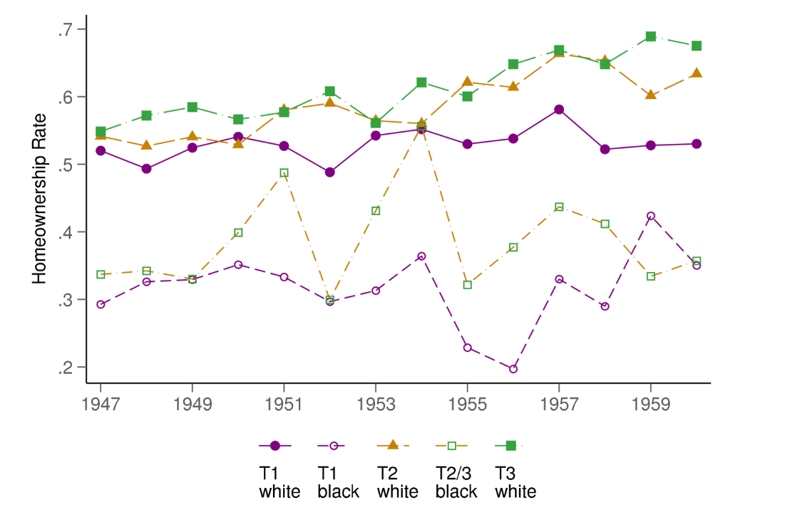
Note: Family income is predicted using the number of earners in the family and the education and occupation of the head. For Black families, the middle and top terciles are combined due to small sample sizes.
Source: Author calculations from the Survey of Consumer Finances 1947-1960.
Finally, we turn to the role of suburbanization. Collins and Margo (2001) attribute a growing black-white homeownership gap from 1940 to 1960 partly to the disproportionate move of white households to the suburbs. It is thus possible that different rates of suburbanization across the income distribution may have contributed to the patterns we describe as well. Indeed, it seems plausible that the expansion in the stock of single-family suburban homes would have benefited higher-income families to a greater extent if these homes tended to be more expensive. Unfortunately, we cannot observe shifts in suburbanization directly in the SCF because suburban status is not measured consistently over time. We can, however, observe whether a recently purchased home is newly built or previously lived-in. Newly built homes are a reasonable proxy for suburban status because they were more likely to be in suburban areas. Specifically, among nonfarm owner-occupied homes built between 1950 and 1960 in the 1960 Census, nearly half were in the suburbs, about one third were in nonmetropolitan areas (which might easily have become suburban in later decades as metropolitan areas expanded), and only 15 percent were in central cities.11 In addition, the median value of new homes in suburban locations was nearly twice as high as the median value of homes in central cities and nonmetro areas, illustrating that purchasing a new suburban home was indeed more expensive than purchasing a home elsewhere.
Table 4 reports the fraction of recent homebuyers in each income group that purchased a newly built home rather than a previously lived-in home. As expected, families in the bottom income tercile were 15 to 20 percentage points less likely to have purchased a newly built home that those in the middle or top tercile. The table also shows that bottom tercile families were a little less likely to have purchased a home at all. Combining these two sets of results, the third row of the table shows that on average only 0.8 percent of the bottom tercile families in the SCF transitioned into a new home in a given year, compared with 2 percent of middle-tercile families and 3 percent of top tercile families.12 Though we lack precise information on the location of residence for the households in our sample, these results are broadly consistent with the idea that the expansion of the suburban housing stock may have helped more families in the upper two terciles transition into homeownership than those in the bottom tercile.
Table 4. Newly-Built Home Purchases by Income Group
| Predicted Income Tercile | |||
|---|---|---|---|
| Bottom | Middle | Top | |
| Percent of recent buyers who purchased a newly-built home | 20.5 | 35.2 | 40.7 |
| Percent of all families that purchased a home (newly-built or previously lived-in) recently | 8.9 | 11 | 12 |
| Percent of all families that purchased a newly-built home recently | 0.8 | 2 | 2.7 |
Note: Recent homebuyers are those who purchased a home in the current or previous year.
Source: Author calculations from the Survey of Consumer Finances 1947-1960.
In sum, the expanding differential in homeownership between lower-income and higher-income families seems to have been partly related to the fact that lower-income families did not have enough income or financial assets to purchase a home. Even though FHA loans had lower downpayment requirements than conventional loans (especially after 1954), FHA mortgages were more often used by middle- and higher-income families. Access to the VA mortgage program, and perhaps access to mortgage credit more generally, may also have played a role. The surge in fertility and the move of middle and higher income households to the suburbs may have contributed to this differential as well. Although our descriptive analysis cannot establish a ranking of the economic significance of these factors, it suggests that—similar to the overall rise in homeownership between 1940 and 1960—the larger increase in homeownership across higher-income groups may also represent the effects of multiple economic forces.
4. Implications for housing wealth
The implications of differential changes in homeownership for wealth depend on how house values and mortgage debt evolved for these groups. The SCF began collecting information on the amount of mortgage debt owed by each family in 1949. Table 5 reports the average house value and average mortgage debt owed by homeowner families by tercile of predicted income for the first three and last three available years in nominal dollars. Average house values increased by the same amount for the top and bottom terciles, and by somewhat more for the middle tercile. Meanwhile, mortgage debt increased by much more in the top two terciles than in the bottom tercile. As a result of these changes, average home equity of homeowner families increased by about the same amount in the bottom two terciles, whereas it increased by less for the top tercile.
Table 5. Changes in Average Home Equity by Tercile of Predicted Income
Dollars
| 1949-51 | 1958-60 | Percent Change | |
|---|---|---|---|
| Average House Value | |||
| Bottom Tercile | $6,704 | $8,802 | 31 |
| Middle Tercile | $8,783 | $12,715 | 45 |
| Top Tercile | $11,995 | $15,680 | 31 |
| Average Mortgage Debt | |||
| Bottom Tercile | $1,226 | $2,032 | 66 |
| Middle Tercile | $2,057 | $4,356 | 112 |
| Top Tercile | $2,684 | $5,399 | 101 |
| Average Equity of Homeowners | |||
| Bottom Tercile | $5,493 | $6,770 | 23 |
| Middle Tercile | $6,736 | $8,359 | 24 |
| Top Tercile | $9,315 | $10,289 | 10 |
| Average Equity of All | |||
| Bottom Tercile | $2,664 | $3,280 | 23 |
| Middle Tercile | $3,551 | $5,090 | 43 |
| Top Tercile | $5,233 | $6,789 | 30 |
Note: Changes in Average Home Equity by Tercile of Predicted Income
Source: Author calculations from the Survey of Consumer Finances 1947-1960.
Combining this information with the average homeownership rates by group (Figure 3), average housing equity increased the most for the middle tercile, reflecting a combination of rising homeownership and rising house values. Meanwhile housing equity increased the least for the lowest income tercile, as homeownership was flat for this group. If we deflate these nominal dollars by the Consumer Price Index, we find that average equity in the bottom tercile increased by only about 4 percent in real terms whereas it increased by a staggering 24 percent for the middle tercile and by about 11 percent in the top tercile. Therefore, gains in real housing wealth were fairly modest at the bottom of the distribution of predicted income, but sizable for the other two groups.
5. Conclusion
The mid-twentieth century was a unique period of rapid expansion in homeownership in America. This analysis documents that the steep rise in homeownership rates was not spread evenly across all types of households but was instead concentrated among those with higher incomes, white collar jobs, and more education. Even though mortgage debt increased substantially over this period, the increases in homeownership combined with increases in house values were enough to lead to notable increases in net housing wealth for these higher-income families—especially for those in the middle part of the income distribution. By contrast, the average net housing wealth of lower-income families increased little during this period in real terms.
Given the significance of owning a home as a source of wealth accumulation for most households (Kuhn et al., 2020), our findings suggest that the rapid yet unequal transformation in homeownership from 1940 to 1960 may have contributed to the rise of the middle class in this period. Future work should consider the significance of these changes for the broader patterns in homeownership, income and wealth inequality over the past 100 years, as well as disentangle the relative importance of the various factors that may have shaped the distribution of housing wealth in America.
References
Aaronson, Daniel, Daniel Hartley and Bhashkar Mazumder, 2021. "The Effects of the 1930s HOLC "Redlining" Maps" American Economic Journal: Economic Policy 13(4): 355-392.
Bailey, Martha J., Melanie Guldi and Brad J. Hershbein, 2014. " Is There a Case for a "Second Demographic Transition"? Three Distinctive Features of the Post-1960 U.S. Fertility Decline. In Human Capital in History: The American Record, edited by Leah P. Boustan, Carola Frydman and Robert Margo, The University of Chicago Press: Chicago.
Benetton, Matteo, Marianna Kudlyak and John Mondragon 2024. "Dynastic Home Equity" Federal Reserve Bank of San Francisco Working Paper Series 2022-13.
Bricker, Jesse, Kevin Moore and Jeffrey Thompson, 2019. "Trends in Household Portfolio Composition" in Handbook of US Consumer Economics, Andrew Haughwout and Benjamin Mandel eds.
Chambers, Matthew, Carlos Garriga and Don E. Schlagenhauf, 2014. "Did Housing Policies Cause the Postwar Boom in Home Ownership?" in Housing and Mortgage Markets in Historical Perspective, Eugene N. White, Kenneth Snowden and Price Fishback, eds.
Collins, William J. and Robert Margo, 2001. "Race and Home Ownership: A Century-Long View" Explorations in Economic History 38: 68-92.
Collins, Wiliam J. and Gregory Niemesh, 2025. "Income Gains and the Geography of the US Home Ownership Boom, 1940 to 1960." in The Economic History of American Inequality, Martha J. Bailey, Leah Platt Boustan and William J. Collins, eds.
Daysal, N. Meltem, Michael F. Lovenheim and David N. Wasser, 2023. "The Intergenerational Transmission of Housing Wealth" NBER Working Paper 31669.
Dettling, Lisa and Melissa Schettini Kearny, 2025. "Did the Modern Mortgage Set the Stage for the US Baby Boom?" NBER Working Paper 33446.
Federal Housing Administration, 1956. Twenty-First Annual Report for the Year Ending December 31, 1954. United States Government Printing Office: Washington.
Fetter, Daniel K., 2013. "How Do Mortgage Subsidies Affect Home Ownership? Evidence from the Mid-Century GI Bills" American Economic Journal: Economic Policy 5(2): 11-147.
Fetter, Daniel K., 2014. "The Twenties Century Increase in U.S. Home Ownership: Facts and Hypotheses" in Housing and Mortgage Markets in Historical Perspective, Eugene N. White, Kenneth Snowden and Price Fishback, eds.
Fishback, Price, Jonathan Rose, Kenneth A. Snowden and Thomas Storrs, 2024. "New Evidence on Redlining by Federal Housing Programs in the 1930s." Journal of Urban Economics 141
Guvenen, Fatih, Fatih Karahan, Serdar Ozkan, and Jae Song, 2021. "What Do Data on Millions of U.S. Workers Reveal About Lifecycle Earnings Dynamics?" Econometrica 89(5): 2303-2339.
Herzog, John P. and James S. Early, 1970. Home Mortgage Delinquency and Foreclosure. National Bureau of Economic Research: New York.
Kuhn, Moritz, Moritz Schularick and Ulrike I. Steins, 2020. "Income and Wealth Inequality in America, 1949-2016" Journal of Political Economy 128(9): 3469-3519.
Rothstein, Richard, 2017. The Color of Law: A Forgotten History of How Our Government Segregated America. Liveright Publishing Corporation.
Sood, Aradhya and Kevin Ehrman-Solberg, 2024. "The Long Shadow of Housing Discrimination: Evidence from Racial Covenants." Working Paper.
1. Carola Frydman, Northwestern University and NBER; Raven Molloy, Federal Reserve Board; Austin Palis, Federal Reserve Board. Return to text
2. Two exceptions are Collins and Margo (2001) who document changes in homeownership by race, and Fetter (2014) who documents changes in homeownership by age. Return to text
3. https://www.archives.gov/research/census/1950/faqs Return to text
4. Specifically, in both years the 95 percent confidence interval around the SCF estimate includes the Census estimate. The nonfarm homeownership rate in the 1950 Census is calculated from Table 2 in Volume 1 of a publication by the Census Bureau https://www.census.gov/library/publications/1953/dec/housing-vol-01.html. Return to text
5. Fetter (2016) attributes part of the increase in homeownership from 1940 to 1945 to rent controls that reduced the profitability of being a landlord and caused landlords to sell their property to owner-occupants. Wartime deaths of young men also likely boosted the aggregate homeownership rate during this period since many of these young men would otherwise have been renters. It is also possible that the VA mortgage program, which began in 1944, could have contributed to boost homeownership rates from 1945 to 1947. Return to text
6. We measure total family income as income obtained from: wages and salaries; boarders; interest, dividends, trust funds and royalties; unincorporated businesses; professional practice, self-employment or farming; pensions; unemployment compensation and welfare; and alimony. For this analysis, we exclude families where the head is retired because in these cases income is a poor measure of permanent income. Moreover, this group did not experience the increase in homeownership seen in the aggregate statistics—its average homeownership rate was relatively constant, at about 67 percent from 1947 to 1960. Return to text
7. The 1940 Census has an indicator for whether an individual earned more than $50 of non-labor income; 27 percent of families with a head in the labor force had such income. Moreover, this type of income was more common for families with less labor income—59 percent of families in the bottom quintile of total labor income had non-wage income. Therefore, using labor income instead of total income would result in material misclassification of families by total income. Return to text
8. Due to changes in the way educational attainment was recorded over time, we are only able to measure education consistently from 1947 to 1960 in three broad categories: no high school, some high school or a high school degree, and any post-high school education. While we would like to include the occupation and education of other adults in the household, this information is not available. Return to text
9. This table limits the sample to families with heads age 35 to 44 because the age distribution of veterans and non-veterans is considerably different. Return to text
10. Other minorities such as foreign-born families from "undesirable" nationality groups experienced discrimination in the mortgage market as well (Rothstein 2017), but the SCF only measures race as White, Black, and other. Return to text
11. Authors' calculations from 1960 Census microdata provided by IPUMS (Ruggles et al. 2025). Return to text
12. The patterns documented in Table 4 are stable over our sample period, which is not surprising since the increase in suburban construction was already underway by the start of our sample period. Return to text
Frydman, Carola, Raven Molloy, and Austin Palis (2025). "Homeownership and Housing Equity in the Mid-Twentieth Century," FEDS Notes. Washington: Board of Governors of the Federal Reserve System, September 24, 2025, https://doi.org/10.17016/2380-7172.3869.
Disclaimer: FEDS Notes are articles in which Board staff offer their own views and present analysis on a range of topics in economics and finance. These articles are shorter and less technically oriented than FEDS Working Papers and IFDP papers.