


FEDS Notes
September 03, 2026
Revisiting the Forecasting Potential of Futures Prices
Alex Haag, Colin J. Hottman, and Amanda Tinkham1
Amid the largest global oil supply shock in history, oil futures prices moved up much less than many expected. The steep backwardation in oil futures from the Strait of Hormuz's closure sparked a spirited debate over whether futures prices were too sanguine about the risks of prolonged disruption. For institutions, including central banks, that use futures as a guide for market expectations of future commodity prices, understanding the performance of futures in forecasting is essential (Bernanke 2008, Baumeister 2023).
In this note, we revisit the forecasting performance of commodity futures prices, using more recent data than prior work such as Reeve and Vigfusson 2011 (PDF) and Baumeister 2023. We find that when the slope of the futures curve is meaningfully different from zero, futures outperform several alternative forecasting approaches, similar to the findings in Reeve and Vigfusson 2011 (PDF). That said, in line with the literature, we also find that futures prices do not in general produce unbiased forecasts.
There are multiple reasons why future commodity spot prices may deviate from those indicated by futures contracts. Fundamentally, futures prices represent the price buyers and sellers agree on today, and this buying and selling is often done to hedge risk, rather than necessarily a bet on where prices will ultimately settle (Vincent and Moore 2026). Storability, inventory dynamics, and arbitrage opportunities also play significant roles in commodity futures price determination (Emmons and Yeager 2002). For storable commodities with sufficiently ample inventories, futures prices should just reflect the spot price plus carrying costs given arbitrage (with the degree of contango or upward slope driven by carrying costs). However, when inventories are low relative to consumption and the convenience yield2 is high, the arbitrage linking futures prices to the cost of carry breaks and the spot price will be higher than futures prices (backwardation). In addition, the market for farther-dated futures prices may be relatively illiquid and fail at times to reflect all relevant market information. Thus, even with rational agents in financial markets, one would not necessarily expect the price of a futures contract with a certain maturity to equal the expected spot price at the time of the contract's expiration. This leads us to the empirical question we investigate: how well do commodity futures do in forecasting future spot prices?
Simple Benchmarks of Forecasting Performance
To evaluate forecast performance, we will compare futures to simple alternative models of future spot prices. The standard benchmark is a random walk-based forecast, which takes today's price as the best approximation of prices in the future $$ (E\left(p_{t+h}\right)=\ p_{t}) $$. Previous research has argued that futures prices often perform no better than a random walk (Alquist et al., 2013).
Another benchmark is a momentum-based forecast (specifically in our case, a random walk with drift in logarithms), which extrapolates forward prices based on recent price changes, with $$ E\left(p_{t+h}\right)=\ p_{t}\ast \left(\frac{p_{t}}{p_{t-h}}\right) $$.
Our final benchmark will be a type of mean-reversion forecast (specifically random walk with mean-reverting increments), which predicts that price changes over time will move toward a long-run average. We assume the long-run average price change is zero and define the mean-reversion forecast by regressing the change in the logged spot commodity price on its lagged log price change and use the resulting negative beta (Table A1) to adjust the recent price change, as follows:
$$$$ ∆_{\_h}{\ln(p}_{t})=\ \ \beta ∆_{\_h}{\ln(p}_{t-h})+\ {\epsilon }_{t} $$$$
$$$$ \textit{where} ∆_{\_h}{\ln(p}_{t})=\ln{\left(p_{t}\right)}-\ \ln{\left(p_{t-h}\right)} $$$$
$$$$ {E(p}_{t+h})=p_{t}\ast {\left(\frac{p_{t}}{p_{t-h}}\right)}^{\beta } $$$$
These forecasting alternatives only incorporate recent historical data3, whereas futures prices potentially incorporate forward-looking information about commodity markets through the futures curve. Given this, when futures prices today are significantly different from spot prices, we might expect futures to perform better at forecasting than backward-looking methods (Reeve and Vigfusson 2011).
Figure 1 provides a graphical example comparison of the forecasting performance of futures against the group of alternative models for the case of Brent oil prices at the 12-month horizon. The y-axis shows the ratio of the 12-month futures price to the spot price in a given month, where values above 1 are when futures are above spot prices (contango) and values below 1 are when futures are below spot prices (backwardation). The blue dots show observations where futures price subsequently outperform all three alternative models in predicting the spot price over the next 12 months, while red dots are when one of the alternative models does better. As you can see in the figure, futures outperform the alternatives particularly when futures prices deviate meaningfully from spot prices (that is, in the extremes of the y-axis). Of course, the figure shows just one commodity and one futures contract maturity.
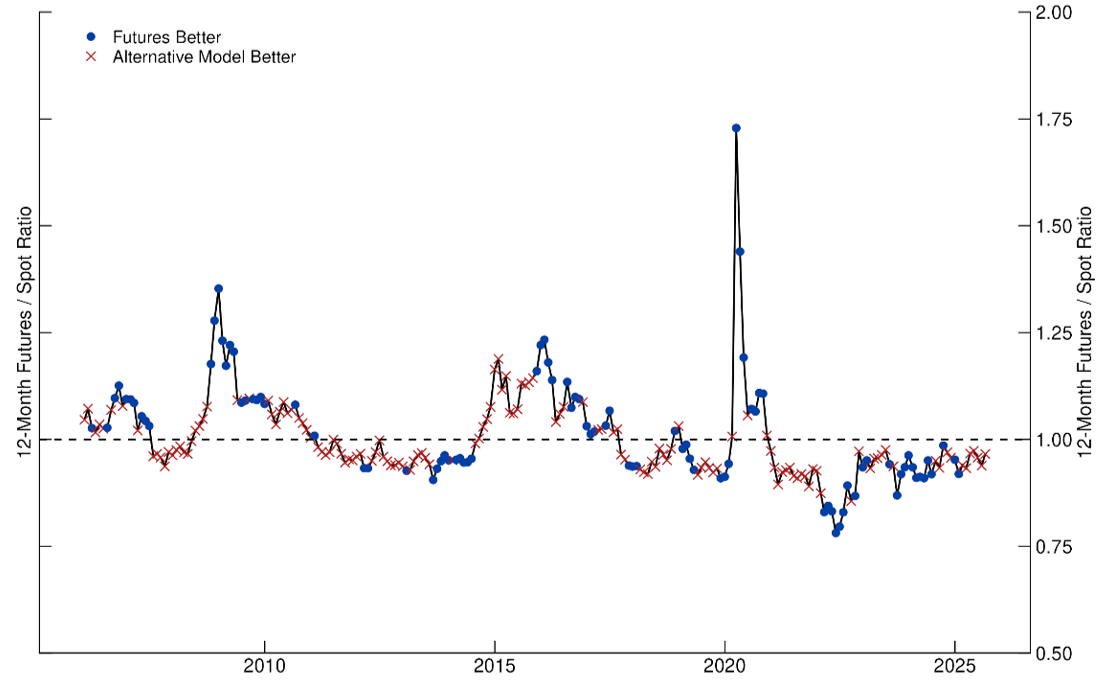
Notes: Alternative models include random walk, momentum, and mean-reversion. The dotted line at 1 represents when 12-month futures and spot prices are the same.
Source: Haver analytics, FRB Staff Calculations.
In the following section, we extend the analysis to the forecasting accuracy of a variety of commodity futures and contract maturities relative to each of the three alternative forecasting methods described above. Our metric is the relative root-mean-squared-error (RMSE) of futures to a given benchmark forecast, where a value less than 1 indicates that futures outperform the alternative forecasting method. We use monthly data on 12 commodities starting in 2005, with the maturing futures contract used to measure the spot price following Baumeister (2023). Futures prices are sampled using the last trading day of each month and correspond to the futures contracts that are 3, 6, and 12 months away, respectively, from the contract measuring spot prices. In the spirit of Reeve and Vigfusson (2011), we bin our results for different slopes of the futures curve and exclude observations in which futures are not materially different from spot prices.
Table 1 shows that when the futures deviate by more than 5 percent from spot prices, futures outperform the random walk forecast for most commodity maturities. Furthermore, this outperformance is quantitatively larger as futures deviate more from spot prices (with the exception of most wheat maturities). That said, it's rare for futures prices in industrial metal commodities in particular to deviate meaningfully from spot prices, as might be expected given they are the most storable commodities in this group.
Table 1: Comparing Futures and Random Walk Commodity Price Forecasts
| Commodity | Maturity | F/S ≤ 0.85 | 0.85 < F/S < 0.95 | 1.05 < F/S < 1.15 | F/S ≥ 1.15 |
|---|---|---|---|---|---|
| Brent | 3-month | 0.87 | 1.02 | 0.64 | |
| 6-month | 0.45 | 0.91 | 0.96 | 0.54 | |
| year-ahead | 0.41 | 0.99 | 0.91 | 0.74 | |
| WTI | 3-month | 0.89 | 1 | 0.56 | |
| 6-month | 0.84 | 1 | 0.55 | ||
| year-ahead | 0.43 | 0.94 | 0.87 | 0.72 | |
| Natural Gas | 3-month | 0.6 | 0.83 | 0.98 | 0.96 |
| 6-month | 0.64 | 0.92 | 1.09 | 0.93 | |
| year-ahead | 0.7 | 0.87 | 1.1 | 1.16 | |
| Gasoline | 3-month | 0.3 | 0.8 | 0.89 | 0.63 |
| 6-month | 0.41 | 0.83 | 0.89 | 0.57 | |
| year-ahead | 0.56 | 0.99 | 0.9 | 0.73 | |
| Corn | 3-month | 0.88 | 1.09 | 1.08 | 0.67 |
| 6-month | 0.53 | 0.94 | 1.03 | 0.74 | |
| year-ahead | 0.85 | 0.84 | 1.03 | 0.82 | |
| Soy | 3-month | 0.38 | 1 | 0.72 | |
| 6-month | 0.54 | 1.01 | 0.86 | ||
| year-ahead | 0.73 | 0.81 | 0.87 | ||
| Wheat | 3-month | 2.47 | 1.44 | 1.13 | 1.37 |
| 6-month | 1.86 | 0.98 | 1.21 | 1.24 | |
| year-ahead | 0.75 | 0.86 | 1.13 | 0.97 | |
| Aluminum | 3-month | ||||
| 6-month | 0.97 | ||||
| year-ahead | 1.55 | 0.95 | |||
| Copper | 3-month | ||||
| 6-month | |||||
| year-ahead | 0.93 | ||||
| Lead | 3-month | ||||
| 6-month | |||||
| year-ahead | 0.72 | 2.17 | |||
| Nickel | 3-month | ||||
| 6-month | |||||
| year-ahead | 1.2 | 1.23 | |||
| Zinc | 3-month | 0.98 | |||
| 6-month | 0.7 | 0.97 | |||
| year-ahead | 0.8 | 0.97 | |||
| Median | 0.7 | 0.97 | 0.96 | 0.74 |
Notes: Table values are relative RMSEs for futures compared to random walk forecasts. A value less than 1 indicates that futures outperform the random walk forecast. The F/S ratio bins are the ratio of forward price to the spot price of each commodity. Year-ahead values are 12 months for energy and metals and 8 months for agricultural products. Empty cells indicate there were no observations in the sample where futures and spot deviated within the specified bin range. Full sample is commodity specific, with the earliest starting in January 2005. All commodities end in April 2026 for the 3-month specification, January 2026 for the 6-month specification, and July 2025 for the 12-month specification for energy and metals and November 2025 for agricultural commodities.
Sources: Haver Analytics, FRB Staff Calculations.
Table 2 shows that, across all commodities and maturities, futures prices meaningfully outperform momentum-based (random walk with drift in logarithms) forecasts. Momentum-based forecasts implicitly assume that recent shocks to demand or supply will be persistent. These forecasts do particularly poorly when there are structural changes in the economic environment or offsetting forces that prevent the persistence of recent shocks. The improvement in forecasting performance of futures over momentum-based forecasts is in most cases significantly more pronounced when futures prices deviate by more than 15 percent from spot prices.
Table 2: Comparing Futures and Momentum-Based Commodity Price Forecasts
| Commodity | Maturity | F/S ≤ 0.85 | 0.85 < F/S < 0.95 | 1.05 < F/S < 1.15 | F/S ≥ 1.15 |
|---|---|---|---|---|---|
| Brent | 3-month | 0.51 | 0.77 | 0.31 | |
| 6-month | 0.14 | 0.61 | 0.62 | 0.24 | |
| year-ahead | 0.13 | 0.64 | 0.75 | 0.46 | |
| WTI | 3-month | 0.47 | 0.75 | 0.28 | |
| 6-month | 0.39 | 0.72 | 0.27 | ||
| year-ahead | 0.15 | 0.53 | 0.64 | 0.46 | |
| Natural Gas | 3-month | 0.51 | 0.67 | 0.69 | 0.65 |
| 6-month | 0.26 | 0.49 | 0.68 | 0.73 | |
| year-ahead | 0.31 | 0.49 | 0.88 | 0.73 | |
| Gasoline | 3-month | 0.18 | 0.48 | 0.83 | 0.36 |
| 6-month | 0.15 | 0.44 | 0.71 | 0.29 | |
| year-ahead | 0.15 | 0.70 | 0.57 | 0.51 | |
| Corn | 3-month | 0.61 | 0.80 | 0.75 | 0.62 |
| 6-month | 0.23 | 0.47 | 0.76 | 0.51 | |
| year-ahead | 0.33 | 0.37 | 0.73 | 0.71 | |
| Soy | 3-month | 0.28 | 0.67 | 0.47 | |
| 6-month | 0.28 | 0.46 | 0.89 | ||
| year-ahead | 0.41 | 0.39 | 1.16 | ||
| Wheat | 3-month | 0.51 | 0.91 | 0.84 | 1.00 |
| 6-month | 0.48 | 0.33 | 0.94 | 0.84 | |
| year-ahead | 0.13 | 0.34 | 0.86 | 0.58 | |
| Aluminum | 3-month | ||||
| 6-month | 0.51 | ||||
| year-ahead | 0.62 | ||||
| Copper | 3-month | ||||
| 6-month | |||||
| year-ahead | 0.44 | ||||
| Lead | 3-month | ||||
| 6-month | |||||
| year-ahead | 0.25 | 1.24 | |||
| Nickel | 3-month | ||||
| 6-month | |||||
| year-ahead | 1.10 | 0.67 | |||
| Zinc | 3-month | 0.72 | |||
| 6-month | 0.76 | 0.69 | |||
| year-ahead | 0.48 | 0.65 | |||
| Median | 0.32 | 0.57 | 0.71 | 0.58 |
Notes: Table values are relative RMSEs for futures compared to momentum-based forecasts. A value less than 1 indicates that futures outperform the momentum-based forecast. The F/S ratio bins are the ratio of the forward price to the spot price of each commodity. Year-ahead values are 12 months for energy and metals and 8 months for agricultural products. Empty cells indicate there were no observations in the sample where futures and spot deviated within the specified bin range. Full sample is commodity specific, with the earliest starting in January 2005. All commodities end in April 2026 for the 3-month specification, January 2026 for the 6-month specification, and July 2025 for the 12-month specification for energy and metals and November 2025 for agricultural commodities.
Sources: Haver Analytics, FRB Staff Calculations.
The comparison of futures to the mean-reversion forecasts (random walk with mean-reverting increments) is shown in Table 3. The medians across commodities and maturities shows futures tend to outperform even against this benchmark, especially with larger deviations of futures from spot prices. That said, futures prices tend to do worse than the mean-reversion forecasts for some commodities such as wheat and most metals maturities (where deviations of futures from spot are more limited).
Table 3: Comparing Futures and Mean-Reversion Commodity Price Forecasts
| Commodity | Maturity | F/S ≤ 0.85 | 0.85 < F/S < 0.95 | 1.05 < F/S < 1.15 | F/S ≥ 1.15 |
|---|---|---|---|---|---|
| Brent | 3-month | 0.86 | 1.01 | 0.72 | |
| 6-month | 0.58 | 0.90 | 0.95 | 0.73 | |
| year-ahead | 0.53 | 0.93 | 0.88 | 0.83 | |
| WTI | 3-month | 0.89 | 0.99 | 0.66 | |
| 6-month | 0.87 | 1.01 | 0.77 | ||
| year-ahead | 0.63 | 0.92 | 0.85 | 0.86 | |
| Natural Gas | 3-month | 0.60 | 0.83 | 0.98 | 0.96 |
| 6-month | 0.76 | 1.00 | 1.12 | 0.98 | |
| year-ahead | 0.88 | 1.01 | 1.15 | 1.15 | |
| Gasoline | 3-month | 0.32 | 0.81 | 0.87 | 0.73 |
| 6-month | 0.62 | 0.91 | 0.87 | 0.95 | |
| year-ahead | 0.71 | 0.93 | 0.98 | 0.84 | |
| Corn | 3-month | 0.89 | 1.06 | 1.08 | 0.68 |
| 6-month | 0.54 | 0.94 | 1.03 | 0.74 | |
| year-ahead | 0.84 | 0.89 | 1.00 | 0.82 | |
| Soy | 3-month | 0.39 | 1.00 | 0.72 | |
| 6-month | 0.58 | 1.05 | 0.82 | ||
| year-ahead | 0.70 | 0.76 | 0.84 | ||
| Wheat | 3-month | 2.35 | 1.38 | 1.12 | 1.38 |
| 6-month | 1.57 | 1.07 | 1.16 | 1.24 | |
| year-ahead | 0.95 | 0.92 | 1.13 | 0.98 | |
| Aluminum | 3-month | ||||
| 6-month | 1.03 | ||||
| year-ahead | 1.15 | 0.98 | |||
| Copper | 3-month | ||||
| 6-month | |||||
| year-ahead | 1.01 | ||||
| Lead | 3-month | ||||
| 6-month | |||||
| year-ahead | 2.11 | 1.38 | |||
| Nickel | 3-month | ||||
| 6-month | |||||
| year-ahead | 1.07 | 1.04 | |||
| Zinc | 3-month | 0.98 | |||
| 6-month | 0.69 | 0.95 | |||
| year-ahead | 0.86 | 0.93 | |||
| Median | 0.74 | 0.99 | 0.98 | 0.86 |
Notes: Table values are relative RMSEs for futures and mean-reversion forecasts. A value less than 1 indicates that futures outperform the mean-reversion forecast. The F/S ratio bins are the ratio of the forward price to the spot price of each commodity. Year-ahead values are 12 months for energy and metals and 8 months for agricultural products. Empty cells indicate there were no observations in the sample where futures and spot deviated within the specified bin range. Full sample is commodity specific, with the earliest starting in January 2005. All commodities end in April 2026 for the 3-month specification, January 2026 for the 6-month specification, and July 2025 for the 12-month specification for energy and metals and November 2025 for agricultural commodities.
Sources: Haver Analytics, FRB Staff Calculations.
While futures show improvement over other simple forecasting methods when futures deviate meaningfully from spot, futures forecasts may still not do particularly well at forecasting future spot prices. In particular, periods where futures substantially deviate from spot prices are generally periods of exceptional uncertainty, such as of supply stress or geopolitical conflict, where forecasting future spot prices is particularly difficult. To show this, we regress the forecast error for the 12-month specification of each method on the slope of the futures curve for Brent:
$$$$ \frac{S_{t+h}-E\left(S_{t+h}^{method}\right)}{E\left(S_{t+h}^{method}\right)}=\ \alpha +\ \beta \left|\frac{F_{t,h}}{S_{t}}\right|-1+\ {\varepsilon }_{t+h} $$$$
where $$ E\left(S_{t+h}^{method}\right) $$ is the forecast of spot for each method described above. A beta coefficient of 0 would indicate forecast errors are independent of the slope of the futures curve. We use the absolute value of the futures/spot ratio since we are only concerned with the deviation from a slope of 0, not the direction (backwardation or contango). Table 4 below confirms that deviations from a futures curve slope of 0 are positively associated with higher forecast errors across all specifications, including futures. So while futures perform better than simple alternatives for Brent, their own forecast errors are also increasing with the futures curve slope.
Table 4: Forecast Errors and the Slope of the Brent Futures Curve
| Random Walk | Momentum | Mean-Reversion | Futures | |
|---|---|---|---|---|
| Futures Curve Slope | 2.092*** | 9.094*** | 1.398*** | 0.787*** |
| (0.323) | (0.597) | (0.316) | (0.296) | |
| Intercept | -0.072** | -0.498*** | -0.04 | 0.011 |
| (0.033) | (0.062) | (0.032) | (0.03) | |
| Observations | 246 | 234 | 246 | 246 |
Notes: Regressions represent the increase in the forecasting error associated with an increase in the F/S ratio. Regression estimates use Newey-West HAC standard errors. P-values are * < 0.1, ** < 0.05, and *** < 0.01.
Sources: Haver analytics, FRB Staff Calculations.
Another way to evaluate the absolute forecast performance of futures prices is to test whether they produce unbiased forecasts. To formally test this, we use the following efficiency regression from the literature:
$$$$ \frac{(S_{t+h} - S_t)}{S_t} = \alpha + \beta \frac{(F_t^h - S_t)}{S_t} + \varepsilon_{t+h} $$$$
where the left-hand side represents the change in the spot price and the right-hand side is the percent deviation of futures from spot in a given period. Given this equation, futures prices would be unbiased predictors of future spot prices under the conditions of alpha equal to 0 and beta equal to 1.
Table 5 shows the results for energy and agricultural commodities of efficiency regressions that explicitly test the null hypothesis of futures being unbiased predictors of future spot prices. Bolded values indicate p-values where the joint hypothesis of alpha = 0 and beta = 1 are rejected at least at the 10% significance level. The results for most commodity-maturity combinations reject that futures prices are unbiased predictors of future spot prices.
Table 5: Efficiency Regressions for Selected Commodities
| $$ \alpha_{3m} $$ | $$ \beta_{3m} $$ | $$ \textit{joint-test}_{3m} $$ | $$ \alpha_{6m} $$ | $$ \beta_{6m} $$ | $$ \textit{joint-test}_{6m} $$ | $$ \alpha_{12m} $$ | $$ \beta_{12m} $$ | $$ \textit{joint-test}_{12m} $$ | |
|---|---|---|---|---|---|---|---|---|---|
| Brent | 0.02 | 1.39 | 0.28 | 0.04 | 1.21 | 0.28 | 0.07 | 1.97 | 0.08* |
| WTI | 0.03 | 1.47 | 0.05** | 0.06 | 1.09 | 0.04** | 0.11 | 1.46 | 0.04** |
| Natural Gas | -0.05 | 0.94 | 0.02** | -0.06 | 0.89 | 0.04** | -0.08 | 0.86 | 0.17 |
| Gasoline | 0.05 | 1.56 | 0.01*** | 0.08 | 1.59 | 0.00*** | 0.14 | 2.32 | 0.02** |
| Corn | 0.00 | 0.53 | 0.03** | 0.00 | 0.79 | 0.57 | 0.02 | 1.07 | 0.87 |
| Soy | 0.02 | 0.81 | 0.08* | 0.05 | 1.03 | 0.08* | 0.10 | 1.77 | 0.09* |
| Wheat | 0.00 | 0.22 | 0.00*** | 0.00 | 0.30 | 0.00*** | -0.02 | 0.68 | 0.16 |
Notes: alpha and beta columns indicate the coefficients from the efficiency regressions. Joint-test columns are the p-value on the joint hypothesis test of alpha = 0 and beta = 1. Regression estimates use Newey-West HAC standard errors. P-values are * < 0.1, ** < 0.05, and *** < 0.01.
Sources: Haver analytics, FRB Staff Calculations.
Conclusion
We find that when the slope of the futures curve is meaningfully different from zero, futures prices generally outperform simple backward-looking methods of forecasting commodity prices. These results suggest that there is important informational content on market expectations reflected in futures prices. That said, our results also caution that futures are typically not unbiased predictors of future spot prices, likely reflecting high uncertainty in periods when futures curves are not flat.
References
Alquist, Ron, Kilian Lutz, and Robert Vigfusson. 2013. "Forecasting the Price of Oil." In Graham Elliott and Allan Timmerman, eds., Handbook of Economic Forecasting, Vol 2A. Amsterdam: Elsevier.
Baumeister, Christiane. 2023. "Measuring Market Expectations." Chapter in Handbook of Economic Expectations by Bachmann R., Topa G., and van der Klaauw, W. Academic Press, 413-442.
Bernanke, Ben S. 2008. "Outstanding Issues in the Analysis of Inflation." Speech at the Federal Reserve Bank of Boston's 53rd Annual Economic Conference, Chatham Massachusetts. June 9.
Emmons, William and Timothy Yeager. 2002. "The Futures Market as a Forecasting Tool: An Imperfect Crystal Ball." Regional Economist, Federal Reserve Bank of St. Louis.
Reeve, Trevor and Robert Vigfusson. 2011. "Evaluating the Forecasting Performance of Commodity Futures Prices (PDF)." International Finance Discussion Papers No. 1025, Board of Governors of the Federal Reserve System. August.
Vincent, Jonathan and Malcolm Moore. 2026. "Why the Oil Futures Curve is not a Crystal Ball." Financial Times, May 15, https://www.ft.com/content/07b8ad0d-86d3-4874-a264-17c34ea3b036?syn-25a6b1a6=1.
Table A1: Beta Coefficients in Mean-Reversion Regressions
| Commodity | $$ \beta_{3m} $$ | $$ \beta_{6m} $$ | $$ \beta_{12m} $$ |
|---|---|---|---|
| Brent | -0.08 | -0.13 | -0.16 |
| WTI | -0.12 | -0.18 | -0.23 |
| Natural Gas | -0.01 | -0.22 | -0.29 |
| Gasoline | -0.15 | -0.34 | -0.2 |
| Aluminum | -0.08 | -0.11 | -0.26 |
| Copper | -0.08 | -0.2 | -0.27 |
| Nickel | 0 | -0.08 | -0.15 |
| Lead | -0.08 | -0.01 | -0.45 |
| Zinc | -0.08 | -0.14 | -0.16 |
| Corn | -0.08 | -0.11 | -0.21 |
| Soy | -0.01 | -0.15 | -0.21 |
| Wheat | -0.09 | -0.14 | -0.09 |
Notes: For 3-month specifications for most metals and corn, 6-month specifications for zinc and wheat, and 12-month specifications for corn and soy, we use the median negative beta coefficient across commodities to impose mean-reversion. Betas are calculated using the full sample for each commodity and maturity, respectively. Full sample for mean-reversion estimates is commodity specific, with the earliest starting in January 2005. All commodities end in April 2026 for the 3-month specification, January 2026 for the 6-month specification, and July 2025 for the 12-month specification.
1. Alex Haag, Colin Hottman, and Amanda Tinkham are with the Board of Governors of the Federal Reserve System. The views expressed in this note are our own, and do not represent the views of the Board of Governors of the Federal Reserve, nor any other person associated with the Federal Reserve System. Return to text
2. The convenience yield is the non-monetary benefit of holding a physical commodity. Return to text
3. For simplicity, we estimate the betas in the mean-reversion specification using the full data sample, which gives the mean-reversion benchmark an advantage since the betas reflect actual future price changes. We could have instead estimated the betas using some type of real-time, expanding-window approach, so that the betas only incorporated historical information. Return to text
Haag, Alex, Colin J. Hottman, and Amanda Tinkham (2026). "Revisiting the Forecasting Potential of Futures Prices," FEDS Notes. Washington: Board of Governors of the Federal Reserve System, September 03, 2026, https://doi.org/10.17016/2380-7172.4171.
Disclaimer: FEDS Notes are articles in which Board staff offer their own views and present analysis on a range of topics in economics and finance. These articles are shorter and less technically oriented than FEDS Working Papers and IFDP papers.