FEDS Notes
May 22, 2018
Shedding Light on Our Economic and Financial Lives
Jeff Larrimore, Alex Durante, Kimberly Kreiss, Ellen Merry, Christina Park, and Claudia Sahm
One way to find out how someone is doing is to simply ask them. If you then want to understand the full range of experience, you have to ask many people, all across the country and from various walks of life. Each year the Federal Reserve does just that with the Survey of Household Economics and Decisionmaking ("SHED"). In November and December of 2017, we interviewed over 12,000 individuals, representative of all adults in the United States, about their economic and financial lives. Here we discuss the responses on three important economic issues: the role of economic conditions in the opioid epidemic, jobs with irregular schedules as a potential barrier to full employment, and how low rates of geographic mobility may relate to family support networks. See our full report, for many more findings on income, work, emergency expenses, higher education, student loans, and retirement savings.
Local Economic Conditions and the Opioid Epidemic
The sharp rise in opioid addiction and overdoses is a subject of national concern, so the 2017 SHED added a question on opioids to explore links to economic well-being.1 One hypothesis, advanced by academics Anne Case and Angus Deaton, is that a long-standing decline in economic opportunities was an important driver of the current opioid epidemic (2017).2 They refer to these as "deaths of despair." Yet, the existing evidence on the role of economic conditions is mixed. For example, Christopher Ruhm (2018) has argued against this hypothesis, using geographic variation in economic outcomes, such as employment and house prices, and opioid-related deaths.3 Similarly, Janet Currie, Jonas Jin, and Molly Schnell (2018) find no clear causal relationship between local employment rates and opioid prescription rates.4 This year's survey attempts to shed light on the debate by linking individual-level exposure to opioid addiction with subjective assessments of local and national economic conditions. There are large differences in exposure to the opioid epidemic by race and ethnicity and smaller differences by economic conditions.
To measure exposure to the opioid epidemic in our survey, individuals report if they "personally know someone who has been addicted to opioids or prescription painkillers."5 This question does not ask specifically about illicit drug use or about an individual's own use of opioids, since individuals might be hesitant to report such behaviors in a survey. By this measure, about one-fifth of adults have been personally exposed to the opioid epidemic. White adults, regardless of education level, are about twice as likely to be personally exposed to opioid addiction as black or Hispanic adults (figure 1).6
Figure 1: Whites more likely than blacks or Hispanics to personally know someone addicted to opioids
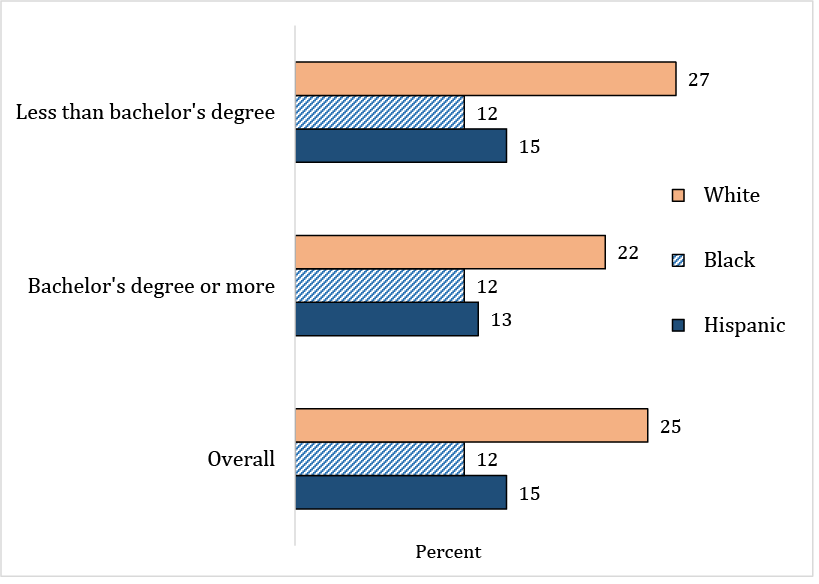
Source: 2017 Survey of Household Economics and Decisionmaking. Note: All pairwise comparisons are statistically different at the one-percent level, except the black and Hispanic rates within and across the two education subgroups.
To investigate the "deaths of despair" hypothesis, figure 2 compares individuals' assessments of local and national economic conditions by their exposure to the opioid epidemic. Adults who have been personally exposed to the opioid epidemic have somewhat less favorable assessments of economic conditions than those who have not been exposed. Among whites, the gap in perceptions of economic conditions by opioid exposure is larger. However, local unemployment rates are similar in the neighborhoods where those exposed to opioids live and where those not exposed live.7 Subjective assessments of economic conditions do show more support for the "deaths of despair" hypothesis than objective outcomes, like local unemployment. Even so, more than half of adults exposed to opioid addiction say that their local economy is good or excellent. Altogether, this analysis suggests that we need to look beyond economic conditions to understand the roots of the current opioid epidemic.
Figure 2: Self-assessment of economic conditions somewhat less favorable among those personally exposed to opioid epidemic
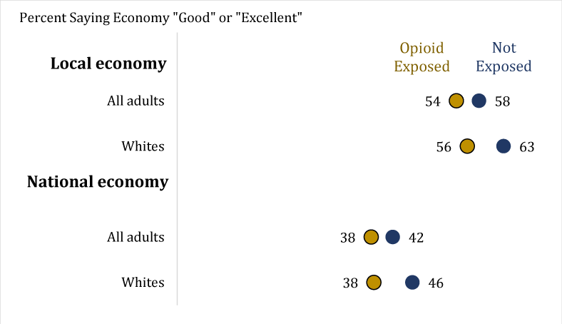
Source: 2017 Survey of Household Economics and Decisionmaking. Note: Estimates in each row are statistically different at the one-percent level.
Irregular Work Schedules and Preferences for Stable Pay
Irregular work schedules, with varying hours from week to week, give employers the ability to match their workforce to shifts in customer demand and other changes in business conditions. Yet work schedules set by employers on short notice may cause financial strain, particularly for low-income workers. In the U.S. Financial Diaries, an ethnographic study of over 200 low- and moderate-income families by Jonathan Morduch and Rachel Schneider, monthly swings in income, even by modest amounts, and unpredictable work hours frequently led to an inability to pay expenses.8 In addition, unpredictable hours may make it difficult for part-time workers to take on additional jobs and increase their family income.
In the survey, more than one-third of non-retirees working part time for economic reasons in 2017 have an irregular work schedule set by their employer (figure 3). One-quarter of non-retired individuals working part time for non-economic reasons, and 12 percent of full-time workers, have such a schedule. This means that many of the part-time workers who would potentially work more hours (and thus are not currently at their full employment) also face the challenge of unpredictable hours. As another sign of differences in employees' status, 3 in 10 of those working part time for economic reasons received a raise in the past year versus more than half of full-time workers who received a raise.
Figure 3: Workers part-time for economic reasons more likely to have irregular schedules and less likely to get a raise
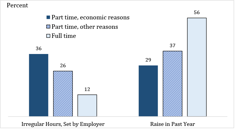
Source: 2017 Survey of Household Economics and Decisionmaking. Note: Among non-retired adults employed for someone else in their main job. Within both hours and raise, the rates for the three employment groups are statistically different at the one-percent level.
Some individuals may be more willing to take on unpredictable hours than others. For example, those with a cushion of savings, fewer fixed expenses, or a greater flexibility, in general, may be willing to exchange stable hours for higher pay or other job characteristics. A hypothetical job choice in the survey suggests that those who actually work irregular hours set by their employers are somewhat more tolerant of varying income than those who actually work regular hours (figure 4). Even with this relationship between actual and hypothetical job choices, it is striking how few individuals would choose the higher pay, varying income job. Only when the varying job pays a lot more, do a majority of non-retirees choose it over the stable-income job. In an experimental setting, Alexandre Mas and Amanda Pallais (2016) found that workers were willing to give up one-fifth of their weekly wages to avoid a work schedule set by their employer with a week's advance notice.9
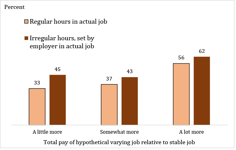
Source: 2017 Survey of Household Economics and Decisionmaking. Note: Among non-retired adults employed for someone else or working as a contractor in their main job. The rates for the two actual job groups are statistically different at the one-percent level for a little more pay and at the five-percent level for somewhat more pay.
Geographic Mobility, Neighborhood Characteristics, and Family Support
Over the past several decades, the rate at which Americans move—both short distances within states and longer distances across the country—has steadily fallen. This reduction in geographic mobility also fits within a pattern of less job switching, more generally, or reduced labor market fluidity, as documented by Molloy and coauthors (2016).10 While the reasons for reduced geographic mobility remain an open question among researchers, evidence is mounting on the importance of local communities on individuals' economic outcomes. As one recent example, Chetty and coauthors (2014) have shown that upward income mobility from one generation to the next varies widely across the country and even within a single metro area.11 This year's survey can also be used to study geographic mobility and to pair it with subjective assessments.
In order to gain insight into geographic mobility, respondents are asked to provide their location when they started high school, which can then be mapped against their current place of residence.12 The distance in miles between the ZIP code where individuals currently live and the ZIP code where they were living in high school is calculated for each survey respondent.13 As figure 5 shows, almost 3 in 10 adults (ages 22 and older) still live in the same ZIP code as where they started high school, and nearly half live within 10 miles. Those who have moved farther away from home are split fairly evenly between distances of 11 to 75 miles, 76 to 500 miles, and more than 500 miles.
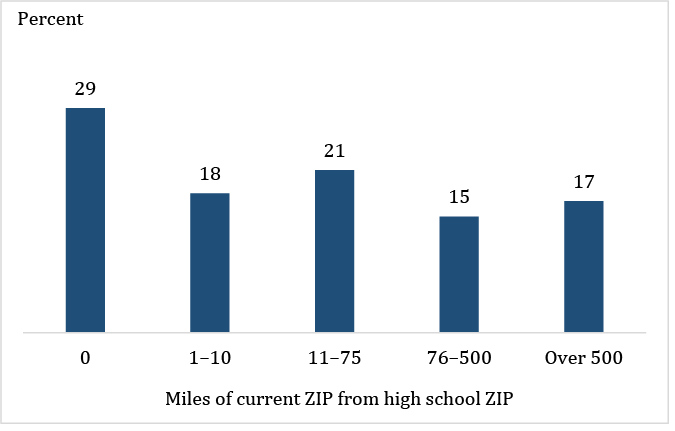
Source: 2017 Survey of Household Economics and Decisionmaking. Note: Among adults age 22 and older.
A major predictor of whether individuals move away from their hometown is their level of education. Three-fifths of adults with a bachelor's degree live more than 10 miles away from where they grew up, versus two-fifths of those who have a high school degree or less. Those who move also have greater levels of income, which is consistent both with their higher education levels and with moving to seek out better economic opportunities.
An additional reason to move away from home would be to live in a community that better fits an individual's preferences and needs than the community that his or her parents had chosen for themselves. While the majority of adults are satisfied with the overall quality of their current neighborhood, those who have moved away from where they grew up are more satisfied with their neighborhood and their housing than those who stayed close to home (figure 6).
Figure 6: Those who have moved more than 10 miles away from home are more satisfied with their neighborhood
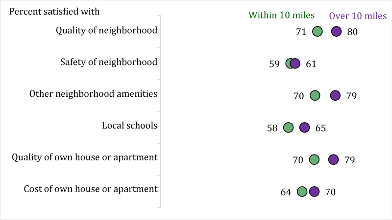
Source: 2017 Survey of Household Economics and Decisionmaking. Note: Among adults age 22 or older. Satisfaction with the cost of own house or apartment excludes those who do not own and are not paying rent. Estimates in each row are statistically different at the one-percent level.
According to a study by the Pew Research Center (2008), family ties are one of the main reasons that people are reluctant to move away from their hometown.14 Likewise, this year's survey shows a similar pattern. Among young adults, in particular, these family ties often come with important financial support. Forty-one percent of young adults (ages 22 to 29) living within 10 miles of where they went to high school either receive financial support from outside their home or are living with others without paying rent (figure 7). Young adults who have moved further away are less likely to receive such support. Financial support from others also declines with age, particularly for those living close to home. These data highlight how family ties and financial support are linked with mobility decisions as individuals enter adulthood.
Figure 7: Young adults who stay close to home much more likely to receive financial support from family and friends than those who move further away
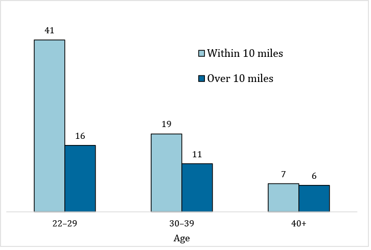
Source: 2017 Survey of Household Economics and Decisionmaking. Note: Among adults age 22 and older. The rates for movers and non-movers are statistically different at the one-percent level at ages 22 to 29 and 30 to 39, but not statistically different for those age 40 and older.
1. See, for example, analysis from the Centers for Disease Control and Prevention on opioid-related deaths, "Understanding the Epidemic," www.cdc.gov/drugoverdose/epidemic/index.html, and the references cited therein for more information. Return to text
2. Anne Case and Angus Deaton, "Mortality and Morbidity in the 21st Century" Brookings Papers on Economic Activity Spring (2017): 397–476. Return to text
3. Christopher J. Ruhm, "Deaths of Despair or Drug Problems?" NBER Working Paper 24188 (2018). Return to text
4. Janet Currie, Jonas Y. Jin, and Molly Schnell, "U.S. Employment and Opioids: Is There a Connection?" NBER Working Paper 24440 (2018). Return to text
5. This question on opioids is modeled after an April 2017 public opinion poll that found 27 percent of adults personally knew someone addicted to opioids (American Psychiatric Association, APA Public Opinion Poll – Annual Meeting 2017, https://www.psychiatry.org/newsroom/apa-public-opinion-poll-annual-meeting-2017). Two other recent surveys found even higher rates of exposure (Robert J. Blendon and John M. Benson, "The Public and the Opioid-Abuse Epidemic" New England Journal of Medicine 378 (2018): 407-411). Return to text
6. Since the measure does not ask about the respondent's own addiction, and instead focuses on addiction among people they know, it may not reflect the ethnicities, education, or geographies of people personally struggling with addiction. Return to text
7. The local unemployment rates, measured with the five-year average from the 2012–16 American Community Survey at the census tract of the respondent, are 7.4 percent for those exposed and 7.3 percent for those who are not. The gap, while still modest, is somewhat larger for the local employment-population ratios for working age adults (age 25 to 64). The local employment-population ratios are 72.7 percent for those exposed to the opioids epidemic and 73.2 percent for those who are not. Return to text
8. Jonathan Morduch and Rachel Schneider, The Financial Diaries: How American Families Cope in a World of Uncertainty (Princeton, NJ: Princeton University Press, 2016); see also the U.S. Financial Diaries website, www.usfinancialdiaries.org/. Return to text
9. Alexandre Mas and Amanda Pallais, "Valuing Alternative Work Arrangements," American Economic Review 107, no. 12 (2017): 3722–3759. Return to text
10. Raven Molloy, Christopher L. Smith, Riccardo Trezzi, and Abigail Wozniak, "Understanding Declining Fluidity in the U.S. Labor Market," Brookings Papers on Economic Activity (Spring 2016), pp. 183–237. Return to text
11. Raj Chetty, Nathaniel Hendren, Patrick Kline, and Emmanuel Saez, "Where Is the Land of Opportunity? The Geography of Intergenerational Mobility in the United States," Quarterly Journal of Economics 129 (December 2014): 1553–1624. Return to text
12. The ZIP code of the current residence is available for all respondents, while the ZIP code of high school residence is available for roughly three-quarters of respondents. The analysis in this box is limited to individuals with both a current and high school ZIP code. Perhaps reflecting that ZIP codes were not introduced until 1963, older respondents are less likely to provide the ZIP code of their high school and will therefore be underrepresented in this analysis. Information on geographic location for individuals is not included in the public-access data set to maintain the privacy of the respondents. Return to text
13. Distance is calculated by matching each ZIP code to latitude and longitude coordinates and then imputing distance using Austin Nichols's Vincenty package in Stata: Austin Nichols "VINCENTY: Stata Module to Calculate Distances on the Earth's Surface," Statistical Software Components S456815 (2003), Boston College Department of Economics, revised February 16, 2007. Return to text
14. D'Vera Cohn and Rich Morin, Who Moves? Who Stays Put? Where's Home? (Washington: Pew Research Center, December 17, 2008), www.pewsocialtrends.org/files/2010/10/Movers-and-Stayers.pdf. Return to text
Larrimore, Jeff, Alex Durante, Kimberly Kreiss, Ellen Merry, Christina Park, and Claudia Sahm (2018). "Shedding Light on Our Economic and Financial Lives," FEDS Notes. Washington: Board of Governors of the Federal Reserve System, May 22, 2018, https://doi.org/10.17016/2380-7172.2192.
Disclaimer: FEDS Notes are articles in which Board staff offer their own views and present analysis on a range of topics in economics and finance. These articles are shorter and less technically oriented than FEDS Working Papers and IFDP papers.