


FEDS Notes
September 03, 2026
Which states are most exposed to tariff increases? A new measure based on the consumption channel
Nick Heyman, Colin J. Hottman, and Ryan Monarch1
Introduction
This note examines the heterogeneous exposure of states in terms of their consumption of direct consumer goods imports, which is an important channel through which states are exposed to increases in trade costs such as tariffs. Building on the methodology that Hottman and Monarch (2020) and Hottman and Monarch (2026) used to construct a similar measure for U.S. income deciles and other demographic groups, we construct a new state-level measure using a recent year of data. We find large differences in exposure across states, document some contributors to these differences, and then conclude with a discussion of the back-of-the-envelope incidence of tariffs implied by them.
1. Heterogeneous Exposure to Imports in Consumption across States
We construct a new measure of the exposure of various U.S. states to direct consumer goods imports in consumption. To do this, we first use the Consumer Expenditure Survey (CES) in 2023 to generate average annual expenditure for representative households in 31 U.S. states (covering 86% of the U.S. population) on consumer product categories.2 Second, we also use state-level import data for 2023 from the U.S. Census Bureau. To filter for consumer goods within the import data, we concord it with the Classification of Broad Economic Categories (BEC) provided by the United Nations Statistics Division and drop HS codes which are not designated as consumption goods. We concord individual product categories in the import data (on an HS code basis) to the CES product categories using an LLM-based concordance of textual descriptions (with Claude Sonnet 4 starting from the concordance in Furman et al 2017). With these two datasets, for each state, we then can generate the fraction of total consumer spending that is on directly imported consumer goods. This allows us to compare differences across states in imported consumption, which are summarized in Figure 1.
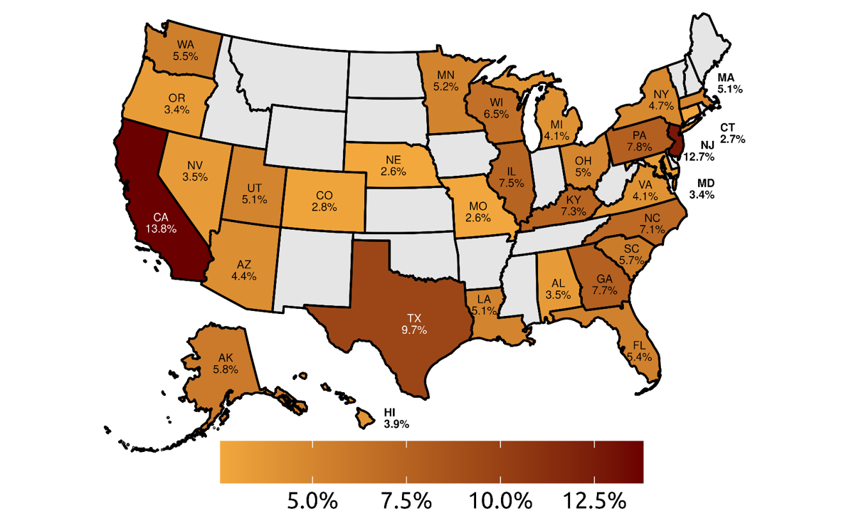
Note: States shown by light gray are not in our sample.
What share of consumption is accounted for by direct consumer goods imports? The shares vary substantially across states. The highest shares of imported consumption are in California (13.8%) and New Jersey (12.7%), while the lowest shares are in Nebraska (2.6%) and Missouri (2.6%). The simple average across our 31 states is 5.6%, while the population-weighted average is 7.1%. These numbers are comparable but smaller than prior estimates of imported consumption nationwide, which are closer to 10% (see, for example, Hottman and Monarch (2020) or Borusyak and Jaravel (2021). However, prior work largely relied on a proportionality assumption, where national-level import penetration rates were combined with differences in consumption at the category-level to estimate heterogenous import exposure across households. Here, our use of state-level import data relaxes this proportionality assumption, with both import data and consumption data directly varying across states. At the same time, since we are now comparing import values measured effectively at wholesale prices to consumption values measured at retail prices, it is not surprising that the import shares of consumption we compute at the state level are on average lower than prior estimates of similar measures at the household income level.3
2. What Explains the Large Differences in Import Exposure across States?
Having shown sizable heterogeneity across states in terms of imported consumption, we next consider potential drivers of that variation due to: A) measurement issues; B) differences in state-level variables such as size and median income; C) differences in the mix of products in the import basket of each state; and D) differences in exposure to various source countries in state imports. We explore each of these in turn.
A. Measurement issues
There are two potential sources of measurement issues that could explain some of the large variation in import shares across states – one in the Consumer Expenditure Survey and the other in the Census state-level import data.
The Consumer Expenditure Survey is only designed to be nationally representative, and state-level estimates could have potentially high variance. We attempted to address this in several ways. First, states were only included if they had more than 300 households responding in the CES (with 80 percent of the 31 included states having more than 500 households). We also scale up CES spending within each state to sum to its PCE total in the BEA's PCE by state data for 2023 (in other words, the CES data are only used to obtain the relative importance of specific product categories, not total state consumer spending). Finally, when identifying direct consumer imports, we dropped any UCC codes appearing in less than two-thirds of our included states (with 119 codes dropped out of 522). Thus, differences in import shares are not primarily driven by some states consuming product categories that other states don't report consuming.
The Census state-level import data are based upon the U.S. state of destination code in electronic entry filings, which is the U.S. state to which the imported merchandise will be ultimately delivered (not the port of entry). These data are used in the literature, for example, in recent work by Rodríguez-Clare et al. (2025). However, in certain cases, this state of destination may reflect a distribution point, from which shipments may later be further distributed to other states. We find that for a small number of product codes (37 UCC codes), the differences across states in implied import shares of consumption were implausibly large. In those cases, product-specific state import shares were replaced by that product's national import share. Thus, our reported differences in total state-level import shares do not reflect extreme differences at the product-level that are likely due to mismeasurement. Although we have attempted to address this, it remains possible that California and New Jersey stand out so much in Figure 1 because they have the two largest ports in the United States, and some shipments that ultimately travel to other states might initially be delivered to distribution points in those two states.
B. State-Level Variation in Size and Income
We use data from the Census Bureau and the BEA on median household income by state, state GDP, and state population and compare it to our estimated spending on imported products. There are strong positive correlations between import spending and both state-level real GDP (0.65) and state-level population (0.65). Thus, larger states (in terms of total economic output or population) have a higher share of consumption coming from direct imported consumer goods than other states, as would be expected from a gravity-type relationship (see Boehm et al. (2026) for evidence of gravity relationships in local U.S. exports). That said, regressing import spending on nominal median household income by state results in a coefficient that is economically small and statistically indistinguishable from zero, which is consistent with the flat import share relative to income that prior work has found (Hottman and Monarch (2020), Borusyak and Jaravel (2021)).
C. Differences in Product Mix of Imports by State
Different states consume products in different proportions, which can explain the differences in import exposure of states. Using CES categories, we separate imported expenditure into 9 broad categories: furnishings and durable household equipment, motor vehicles and parts, recreational goods and vehicles, other durable goods, clothing and footwear, food and beverage purchases, gasoline and other energy goods, and other nondurable goods. To investigate variation systematically, we use a regression-based variance decomposition as in Hottman et al. (2016) to attribute the variance in import shares across states into the contributions of our product buckets to that variance, with the results shown in Table 1. For example, we find that differences in imported spending on "other durable goods", a catch-all category that include items such as cellphones, explains about 24 percent of the variance in state-level import shares, while "food and beverages" and "furnishings and household equipment" each explain about 14 percent. Thus collectively, differences in those three categories alone explain more than 50 percent of the variance in import shares of consumption across states.
Table 1: Import Product Mix Variance Decomposition
| Other Durable Goods | Food and beverages | Furnishings and household equipment | Other nondurable goods | Motor vehicles and parts | Gasoline and other energy goods | Clothing and footwear | Recreational goods and vehicles | Residual products | |
|---|---|---|---|---|---|---|---|---|---|
| Share of variance (%) | 24.3 | 13.8 | 13.5 | 11.2 | 10.2 | 9.3 | 7 | 5.2 | 5.5 |
D. State Differences in Exposure to Source Countries
In their import basket, U.S. states are also differentially exposed to different source countries. For example, we estimate that almost 29% of Illinois's imports come from China, while only about 9% of Massachusetts's imports come from China. We again conduct a variance decomposition, this time into major trading partners and country groupings, with the results reported in Table 2. We find that differences in imported spending from China explains about 24 percent of the variance in state import shares, while the EU explains about 19 percent and Mexico about 15 percent. Collectively, differences in imported spending on those three countries explain almost 60 percent of the variance of import shares across states. Interestingly, differences in imported spending from Canada only explain about 2 percent of the variation.
Table 2: Import Source Country Variance Decomposition
| China | EU | Mexico | Japan + S. Korea + Taiwan + Singapore | Vietnam + Thailand + Malaysia + Indonesia | India | UK | Canada | Brazil | Residual countries | |
|---|---|---|---|---|---|---|---|---|---|---|
| Share of variance (%) | 24.3 | 19.2 | 14.8 | 8.3 | 8.1 | 6.1 | 2.2 | 1.6 | 1 | 14.5 |
Note: share doesn't sum exactly to 1 due to rounding.
3. Heterogeneous Effects of (Uniform) Trade Policy
Finally, we present back-of-the-envelope estimates of the incidence of tariffs across states implied by our calculations. Although recent tariff increases have not been applied uniformly across all U.S. imports, we nevertheless approximate the recent tariff actions as a uniform 10 ppt. tariff increase on all U.S. imports of final goods for the purpose of illustrating the potential differences in direct state-level exposure.4 In this exercise, we also assume for illustrative purposes that this uniform tariff passes through fully to consumer prices. Given these simplifying assumptions, and with our state-level import data as a share of consumption, it is straightforward to identify which states are most affected by the tariff: those with the highest shares of imports.
As can be seen from Figure 1, with uniform tariff increases on all products, households in California, New Jersey, Texas, and Pennsylvania would be most affected, while households in Nebraska, Missouri, Connecticut, and Colorado would be least affected. Quantitatively, our simplifying assumptions imply that California would experience an increase in its cost of living of about 1.4 percent and Pennsylvania would experience a cost of living increase of about 0.8 percent, while Nebraska would experience a cost of living increase of only about 0.3 percent. Thus, we find large differences across U.S. states in terms of their direct cost of living exposure to a uniform U.S. tariff increase. Of course, our earlier variance decompositions imply that non-uniform, sector- and country-specific tariffs would also be expected to lead to sizable differences in effects across states.
References
Boehm, Christoph E., Aaron Flaaen, Nitya Pandalai-Nayar, and Jan Schlupp, "The local-area incidence of exporting", Journal of International Economics, 2026, Vol. 161.
Borusyak, Kirill, and Xavier Jaravel, "The Distributional Effects of Trade: Theory and Evidence from the United States", NBER Working Paper 28957, 2021.
Furman, Jason, Katheryn N. Russ, and Jay Shambaugh, "U.S. Tariffs are an Arbitrary and Regressive Tax", VoxEU.org, 2017.
Hottman, Colin J., and Ryan Monarch, "A matter of taste: Estimating import price inflation across U.S. income groups", Journal of International Economics, 2020, Vol. 127.
Hottman, Colin J., and Ryan Monarch, "Oh, Give me a Home (Trade Share): Differential Import Price Inflation and Gains from Trade Across U.S. Households", Working Paper, 2026.
Hottman, Colin J., Stephen J. Redding, and David E. Weinstein, "Quantifying the Sources of Firm Heterogeneity", Quarterly Journal of Economics, 2016, Vol. 131, No. 3.
Minton, Robbie, and Mariano Somale, "Detecting Tariff Effects on Consumer Prices in Real Time", FEDS Notes, Washington: Board of Governors of the Federal Reserve System, 2025.
Rodríguez-Clare, Andrés, Mauricio Ulate and Jose P. Vasquez, "The 2025 Trade War: Dynamic Impacts Across U.S. States and the Global Economy", NBER Working Paper 33792, 2025.
1. Nick Heyman and Colin J. Hottman: Board of Governors of the Federal Reserve System (emails: [email protected] and [email protected]). Ryan Monarch: Syracuse University (email: [email protected]). The views expressed are solely the responsibility of the authors and should not be interpreted as reflecting the views of the Board of Governors of the Federal Reserve System or any other person associated with the Federal Reserve System. Return to text
2. At the time we started this work, 2023 was the latest year available in the Consumer Expenditure Survey. We focus on 31 U.S. states given data availability, as discussed in section 2.A. Return to text
3. We could use the PCE bridge tables to add on a retail margin to the import values and thus scale up our import shares, but we chose not to do so in order to be consistent with the margin-related passthrough assumptions discussed in Minton and Somale (2025). Return to text
4. For simplicity, this analysis ignores indirect exposure via tariffs on upstream intermediate inputs that are incorporated into downstream final consumer goods. Since they don't include these indirect imports, our import shares are a lower bound on the total share of imports in consumption. And all else equal, including tariffs on indirect imports would increase the cost of living effects we discuss. Return to text
Heyman, Nick, Colin J. Hottman, and Ryan Monarch (2026). "Which states are most exposed to tariff increases? A new measure based on the consumption channel," FEDS Notes. Washington: Board of Governors of the Federal Reserve System, September 03, 2026, https://doi.org/10.17016/2380-7172.4157.
Disclaimer: FEDS Notes are articles in which Board staff offer their own views and present analysis on a range of topics in economics and finance. These articles are shorter and less technically oriented than FEDS Working Papers and IFDP papers.