IFDP Notes
January 19, 2018
Understanding Global Volatility
Juan M. Londono and Beth Anne Wilson *
Volatility has been at historically low levels of late for a wide range of risky assets, not just in the United States but across most international markets. The broad-based nature of low volatility is not surprising given that volatility measures tend to track each other closely. In particular, for stock markets, option-implied volatility (of which the VIX, the option-implied volatility of the S&P 500, is the best known measure) is strongly correlated across countries (figure 1), suggesting a sizable global component to volatility. In this note, we identify a global component of equity option-implied volatilities and address two questions: What are its fundamental drivers? And, given these drivers, are recent levels of volatility unexpectedly low? We find that global factors and U.S. conventional and unconventional monetary policies are key to understand the dynamics of global volatility and that these factors can largely account for the recent low levels of global volatility.
Our measure of global implied volatility is calculated as the market-value-weighted average of the equity option-implied volatility for representative indexes in the United States, the United Kingdom, Germany, Japan, France, the Netherlands, and Switzerland.1 Table 1 shows the correlations among all countries' implied volatilities and with global volatility. Indeed, as the high values of correlations show, the global component accounts for most of the variation of each country's measure.
What are the fundamental drivers of global volatility?
A number of factors could affect the volatility of global stock markets, including current economic conditions; conventional and unconventional monetary policies; economic, geopolitical, and policy uncertainty; and the expected probability of recessions. To capture these factors, we examine a wide range of U.S. and non-US variables. Two issues need to be addressed when evaluating the importance of these variables. The first is the problem of endogeneity between the drivers and volatility; for example, how are we sure that fear of a recession increases volatility and not the other way around? The second is the persistent nature of global volatility, or the fact that volatility is a slow moving variable so that its value today is, in general, a very good guess of what it will be tomorrow. To deal with these issues, we run a series of vector autoregressions (VARs) with the proposed variables and global volatility.2 We estimate the system of equations using monthly data from January 2000 to August 2017 and use a variety of statistical criteria to select variables with the most explanatory power for global volatility.3
We identify eight variables as being the most important drivers of global volatility and divide these into three sets. The first set corresponds to U.S. economic and risk variables: U.S. industrial production (IP) growth; the expected probability of a U.S. recession occurring within the next quarter, as measured by the Survey of Professional Forecasters (SPF); and the U.S. economic policy uncertainty index (EPU) developed by Baker, Bloom, and Davis (2016) using newspaper coverage. The second set captures U.S. monetary policy: the Fed funds rate when this rate is above zero and the shadow Fed funds rate (Wu and Xia, 2016) in the period where the zero-lower-bound is binding to capture the effects of unconventional policies. From the fourth quarter of 2008 onwards, the ratio of total assets of the Federal Reserve as a share of U.S. GDP also proved important in capturing the effects of unconventional policy and was included. The third set captures global factors: non-US IP growth, the global EPU index, and the expected probability of recessions outside of the United States within the next 12 months, a measure calculated by Board staff using foreign economic and financial indicators (Cuba-Borda, Mechanik, and Raffo, forthcoming).
We use a variance decomposition approach to assess the relative importance of these drivers in explaining volatility. When using a VAR setting, the standard way to measure how much each variable (or set of variables) adds to the fit is to look at the forecast error variance. Figure 2 shows the portion of the 6-month ahead forecast error variance of global volatility and, for comparison, of the U.S. option-implied (VIX), explained by each of the three sets of drivers. The eight drivers in all three sets together account for between a third and a half of the forecast error variance of global and U.S. option-implied volatility, with the most important drivers being the global variables. The remaining fraction of the variance forecast is explained by own shocks to the global volatility and VIX, respectively. Thus, according to this analysis, global factors, on top of U.S. variables, would appear to be key in understanding not only the dynamics of global volatility but also of the VIX.
Is recent volatility unexpectedly low?
Global volatility was near 20 percent at the end of 2015, close to its mean value over the period from 2000 to 2017, but by mid-2017 it had almost halved. To judge how well this decline is explained by the sets of drivers in our analysis, we estimate the following three models: (i) with U.S. variables only but excluding U.S. monetary policy variables, (ii) with all U.S. variables, including conventional and unconventional U.S. monetary policies, and (iii) the full set of variables including global drivers and all U.S. variables. We estimate the models for a sample ending in December 2015, right before the recent period of relatively low volatility. In-sample, all models fit global volatility quite well, which is due, in part, to the very persistent nature of global volatility, as captured by the importance of the lagged dependent variable.
To see how well the fundamental determinants explain the recent reduction in volatility, we perform an out-of-sample exercise for global volatility and, for comparison, also for the VIX. Figure 3 shows how global volatility and the VIX would have evolved since January 2016 under each model, assuming that the values of the determinants (such as domestic and foreign economic growth, monetary policies, and EPU indexes) are known each period. The U.S. model without monetary policies does a poor job of matching the recent behavior of volatility. The U.S. with monetary policy model does a somewhat better job, but it is the global model that best explains the reduction in both global volatility and the VIX since January 2016. In fact, the global model would suggest that neither global volatility nor the VIX are unexpectedly low once the effects of global variables and U.S. monetary policies are taken into account.
There has been a lot of discussion about whether realized volatility is also too low, and how this is a potential explanation for the low implied volatility.4 To assess this, we extend the out-of-sample exercise to understand the fundamental drivers of the recent decrease in global realized volatility (figure 4). Again, global variables, on top of U.S. monetary policies, explain well the reduction in global realized volatility.
Our research suggests that favorable economic and financial conditions abroad and the reduced probability of foreign recessions as well as accommodative monetary policies in the United States are key to understand the recent episode of low implied and realized global and U.S. equity market volatility.
Table 1
| Global volatility | U.S. (VIX) | Germany (VDAX) | Japan (VXJ) | U.K. (VFTSE) | Switzerland (VSMI) | |
|---|---|---|---|---|---|---|
| Global volatility | 1 | |||||
| U.S. | 0.98 | 1 | ||||
| Germany | 0.85 | 0.86 | 1 | |||
| Japan | 0.8 | 0.82 | 0.73 | 1 | ||
| U.K. | 0.93 | 0.95 | 0.94 | 0.79 | 1 | |
| Switzerland | 0.87 | 0.88 | 0.95 | 0.8 | 0.95 | 1 |
Notes: Table 1 shows the unconditional correlation between the global volatility and the option-implied volatility of the following countries' representative indexes: the United States, Germany, Japan, the United Kingdom, and Switzerland. The table also show the correlation between the implied volatility of each pair of countries.
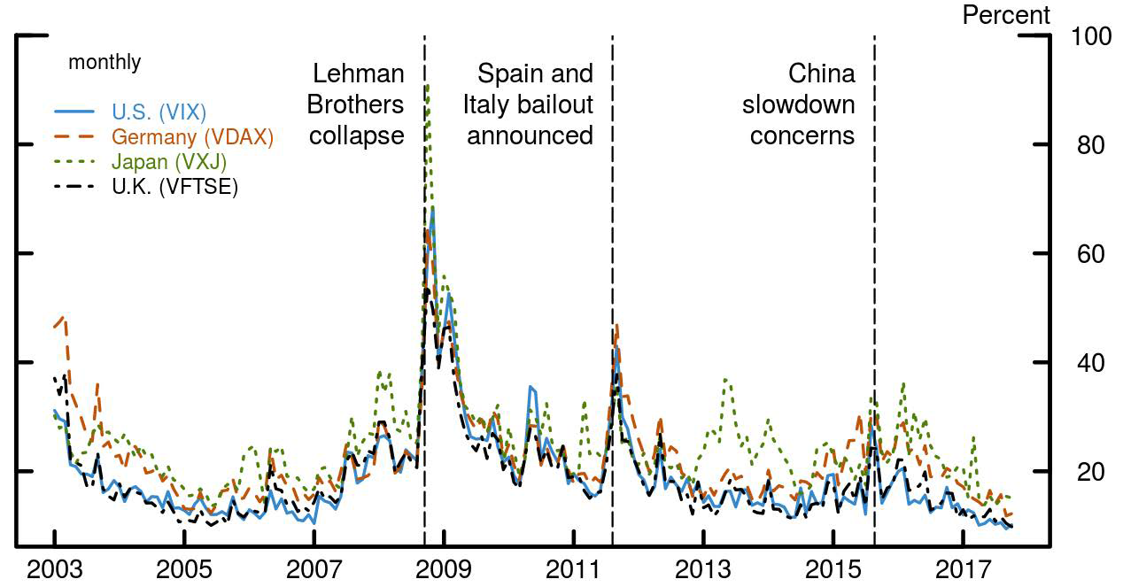
Notes: Figure 1 shows the time series of the 30-day option-implied volatility for the representative index of the United States (solid blue line), Germany (dashed orange), Japan (dotted green), and the United Kingdom (dot-dashed black) between January 2003 and August 2017. To illustrate the effect of key developments on all countries' volatility, we mark the following events (vertical lines): the collapse of Lehman Brothers on September 2008, the announcement of the bailout of Spain and Italy on June 2012, and March 2015, when concerns about China's economic slowdown dominated the headlines.
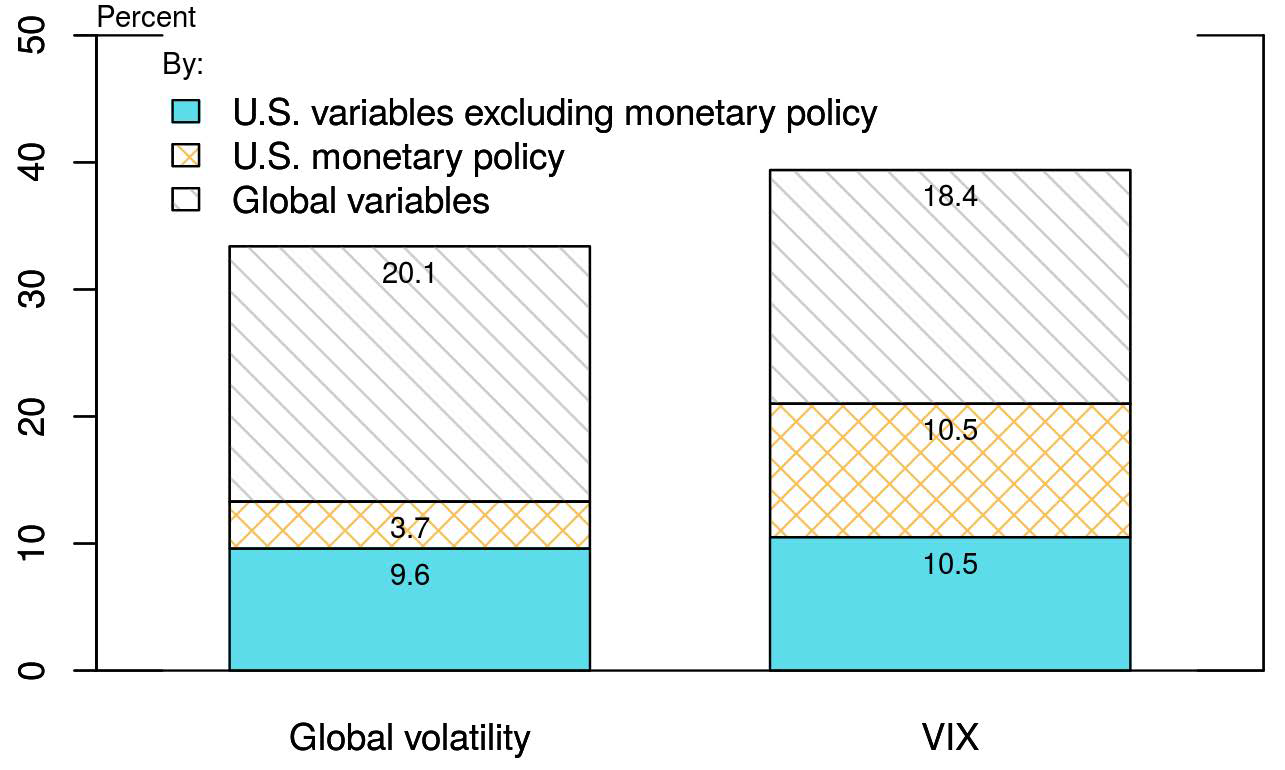
Notes: Figure 2 shows the portion of the 6-month ahead forecast error variance of global volatility (left bar) and the VIX (right bar) explained by the following sets of variables: U.S. variables excluding monetary policy (lower portion of the bars in blue), U.S. monetary policy (mid portion in orange), and global variables (upper portion in grey).
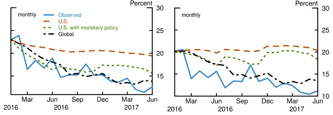
Notes: Figure 3 shows the out-of-sample forecast of the global implied volatility (left panel) and the VIX (right panel) when the fundamentals drivers are known each period. The solid blue line shows the time series of the observed time series, the dashed orange line shows the out-of-sample forecast for the U.S. model without monetary policy, the dotted green line shows the forecast for the U.S. with monetary policy model, and the dot-dashed black line shows the forecast for the model with all variables (global model).
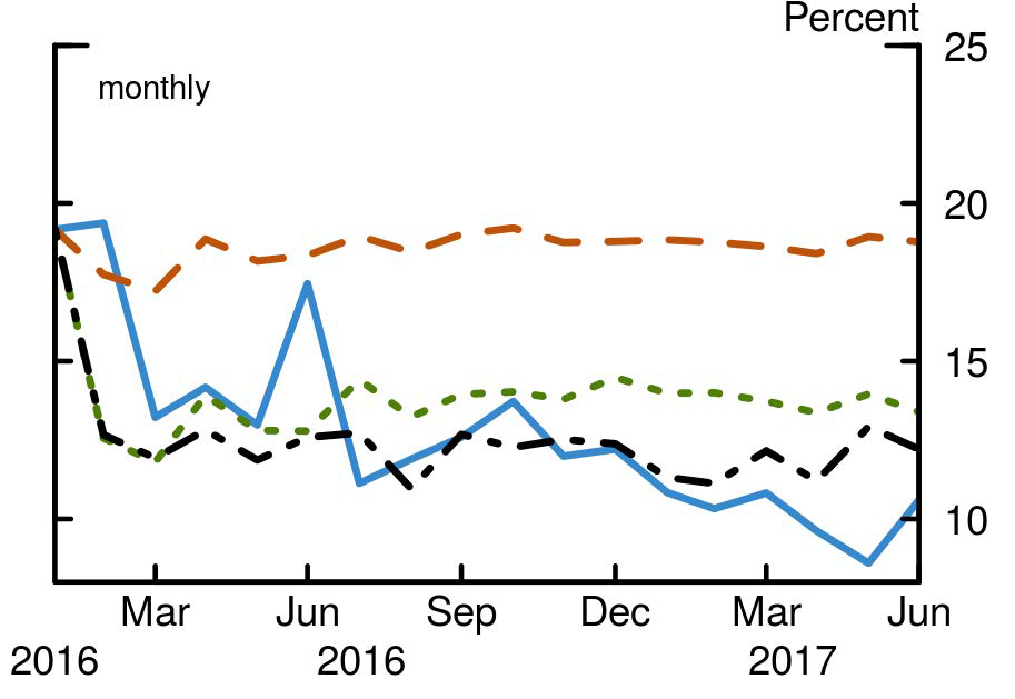
Notes: Figure 4 shows the out-of-sample forecast of the global realized volatility, which is calculated as the market-value-weighted average of all countries' realized volatility, when the fundamentals drivers are known each period. The solid blue line shows the time series of the observed time series, the dashed orange line shows the out-of-sample forecast for the U.S. model without monetary policy, the dotted green line shows the forecast for the U.S. with monetary policy model, and the dot-dashed black line shows the forecast for the model with all variables (global model).
Bibliography
Baker, S. R., Bloom, N., and Davis, S. J. (2016), "Measuring Economic Policy Uncertainty," The Quarterly Journal of Economics 131 (4):1593-1636.
Bollerslev, T., Marrone, J., Xu, L., and Zhou, H. (2014), "Stock Return Predictability and Variance Risk Premia: Statistical Inference and International Evidence," Journal of Financial and Quantitative Analysis 49 (3): 633-661.
Cuba-Borda, O., Mechanik, A., and Raffo, A. (forthcoming), "Monitoring the World Economy: A Global Condition Index," International finance Discussion Paper Notes, Federal Reserve Board of Governors.
Wu, J. C. and Xia, F. D. (2016), "Measuring the Macroeconomic Impact of Monetary Policy at the Zero Lower Bound," Journal of Money, Credit and Banking Vol. 48, No. 2–3: 253-291.
* Juan M. Londono ([email protected]) is a Principal Economist in the International Financial Stability Section and Beth Anne Wilson ([email protected]) is a Deputy Director in the Division of International Finance, Board of Governors of the Federal Reserve System, Washington, D.C. 20551 U.S.A. We thank Nathan Mislang for excellent assistance, and Shaghil Ahmed, Stephanie Curcuru, Eric Engstrom, Ricardo Correa, and Steve Kamin within the Federal Reserve Board for their comments. The views in this paper are solely the responsibility of the authors and should not be interpreted as reflecting the views of the Board of Governors of the Federal Reserve System or of any other person associated with the Federal Reserve System. Return to text
1. Perhaps the most intuitive method to identify global volatility is to estimate the first principal component, which is a linear combination of the individual series with weights calculated to account for as much of their variability as possible. In this case, however, implied-volatility series are so highly correlated that simpler aggregation methods, such as weighted averages, yield a common component almost identical to the first principal component. Using the weighted average facilitates the interpretation as it keeps the same units as those of volatility (that is, in percent) and resembles aggregation methods for volatility previously used in the literature (see, for instance, Bollerslev et al. 2014). Return to text
2. To identify the impact of each variable, we order the variables in the VAR assuming the direction in which they cause each other. In particular, as it is common in the literature, economic activity measures are the most exogenous variables, followed by monetary policy, uncertainty measures, and global volatility, the most endogenous variable. This represents just the contemporaneous causal ordering; all variables are allowed to affect each other with a lag. Return to text
3. In particular, in variable selection, we take into consideration the gains in R2 for the global volatility equation when each variable is added; the proportion of the three-month and six-month ahead forecast error variance of global volatility explained by each variable; and the maximum response of global volatility to a shock in each variable and whether this response is statistically significant. Return to text
4. Option-implied volatility has two components: the expected realized variance and a variance risk premium. Intuitively, one could think of the amount investors are willing to pay to avoid extreme outcomes in equity markets as being a function of their expectations based on past volatility of markets and on how much they are willing to pay to avoid volatility risk. Return to text
Londono, Juan M. and Beth Anne Wilson (2018). "Understanding Global Volatility," IFDP Notes. Washington: Board of Governors of the Federal Reserve System, January 2018, https://doi.org/10.17016/2573-2129.40.
Disclaimer: IFDP Notes are articles in which Board economists offer their own views and present analysis on a range of topics in economics and finance. These articles are shorter and less technically oriented than IFDP Working Papers.