FEDS Notes
November 05, 2021
Differences in Rent Growth by Income 1985-2019 and Implications for Real Income Inequality
Daryl Larsen, and Raven Molloy*
Introduction
Large and growing income differentials in the US have generated a mounting interest in income inequality among economists. The average income in the highest quintile of households increased by about 70 percent in real terms from 1985 to 2019, whereas the average income of the lowest quintile only increased by 20 percent during this period (Semega et al. 2020). However, these estimates of real incomes use the same price index to deflate nominal incomes, which requires the assumption that all households faced the same changes in the prices of goods and services that they purchase. Differences in the types of goods and services consumed, the geographic location of the purchase, or the type of store or outlet where purchased could all contribute to meaningful differences in price inflation faced by households in different income groups.
This note takes a step towards measuring differential inflation rates across income groups by examining how quality-adjusted changes in rent have differed for households across the income distribution from 1985 to 2019. Rent is an especially important component of household spending to consider because housing services account for more than 25 percent of the household spending basket in the Consumer Price Index, and the price of housing services is measured using rent.1 Moreover, it would not be surprising to find material differences in rent growth across the income distribution, since housing costs have been rising more in locations where high-income households tend to live. For example, Moretti (2013) finds that rent growth from 1980 to 2000 was faster in metropolitan areas where college-educated people tend to live than in those where high-school educated people tend to live.
We measure the rent changes facing households in different income groups by calculating changes in rent for individual housing units in the American Housing Survey and grouping rent growth observations according to the income of the resident. We find that rent growth differentials across groups were fairly minor overall. Rent growth was slightly faster for households at the top of the income distribution from 1985 to 2001, but this differential disappeared in the second half of the sample. Cumulating over the entire period, rent increased by 81 percent at the top quintile, and by 72 percent at the bottom quintile.
To assess the implications for a general measure of inflation, we allow the price of housing services to vary by income quintile and assume that the prices of all other goods and services are the same across groups. We also allow the expenditure share on housing services to vary by income quintile, since lower income households tend to spend a larger fraction of their consumption on housing than higher income households. In the first half of our sample, the differences in consumption baskets roughly offset the differences in rent growth across groups, leading to essentially no difference in general price inflation by income. In the second half of the sample, we estimate slightly higher inflation for lower income groups owing to their larger share of housing services. Cumulating over the entire period, the general price index rose by 136 percent for the top income quintile and by 143 percent for the bottom quintile. These differences are fairly minor relative to the widening in nominal income inequality during this period. Thus, on the whole, we find that accounting for differences in the price of housing services faced by households at different income levels does not change the conclusion that real income inequality expanded substantially over the past three decades.
The Case for Examining Rent
Even though only about one-third of households are renters, the Consumer Price Index uses rent to estimate changes in the price of housing services for all households because the price of housing services is not directly observable for owner-occupants.2 Specifically, for owner-occupied homes changes in rent of tenant-occupied units are weighted to more closely reflect the owner-occupied stock. In practice, this re-weighting has had little effect on the long-run trends in the estimated price of housing services. The index for rent paid by tenants increased by an average annual rate of 3.2 percent from 1985 to 2020, while the index for owners' equivalent rent increased by an average annual rate of 3.1 percent over this period. Consequently, in this note we will use rent paid by tenants to proxy for the price of housing services of all households, whether renters or owner-occupants.
One concern with the focus on rent is that there are fewer renters in higher segments of the income distribution. As shown by Figure 1, only 12 percent of households in the top income quintile in 2019 were renters. Because renting is so uncommon for this group, the rents that are observed may be a poor proxy for the price of housing services of owner-occupied homes in this group. Indeed, research has found that the ratio of rent to prices tends to be lower for high-value homes, signaling that these two types of units may not be comparable for high-income households (Garner and Verbrugge 2009, Heston and Nakamura 2009). That said, because the average growth rate of owners' equivalent rent was almost the same as the average growth rate of tenants' rent over our sample period, we maintain that changes in the rents paid by high-income households should provide a reasonable proxy for the changes in the price of housing services at the top of the income distribution, at least for the purpose of calculating long-run average growth rates in a CPI-type framework.
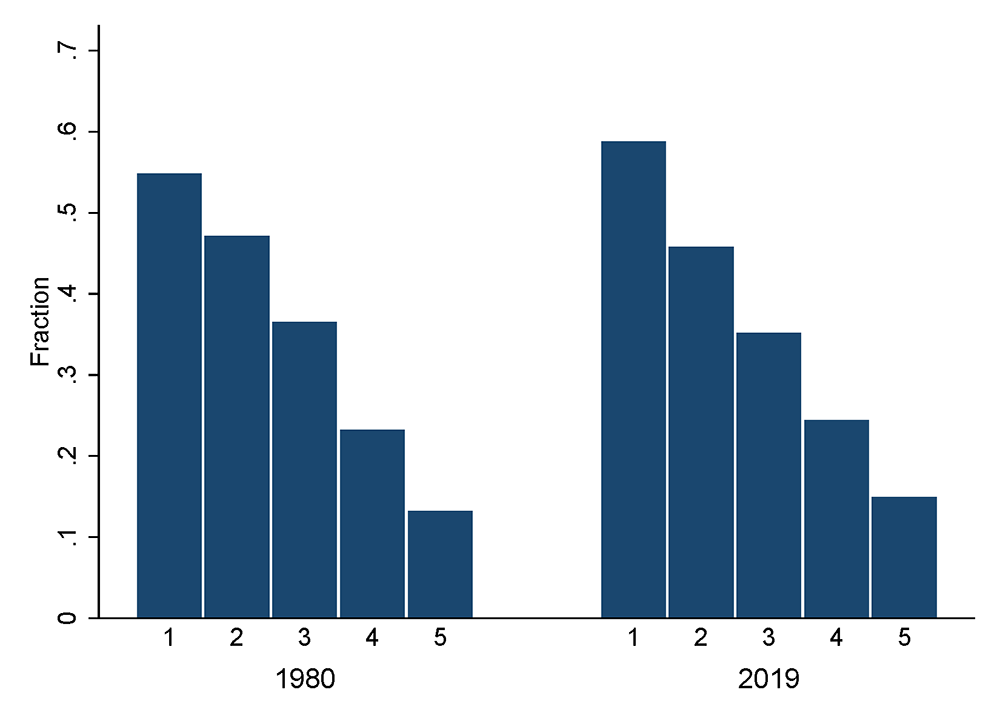
Source: 1980 Census and 2019 American Community Survey. U.S. Census Bureau. https://www.census.gov/programs-surveys/acs.
Rent in the American Housing Survey
The American Housing Survey is a nationally-representative panel that tracks housing units over time. We calculate the annual rent payments for each renter household based on the reported rent and reported frequency of rent payments.3 To establish some basic facts about rent payments across the income distribution, we first regress the natural logarithm of rent on a set of indicators for each quintile of the income distribution, omitting the bottom quintile. The regression also includes a set of year indicators to abstract from the general rise in prices. The first column of Table 1 reports the results and shows that higher income households tend to pay much higher rent than lower income households. Of course, higher income households live in larger, higher quality housing units so one should not interpret these results as reflecting differences in the price of housing services. In the second column, we add controls for housing characteristics such as unit size, number of bathrooms, and the resident's rating of unit quality. These controls reduce the rent differentials across groups, but they are still large. These results suggest that households in higher income groups pay significantly more rent than households in lower income groups, even for a similar quality of housing. However, higher income households may be located in areas with higher quality amenities, in which case the higher rents would be providing them with a greater quantity of housing services. The AHS is only large enough to identify 15 metropolitan areas in all of the survey years. As shown in column 3, adding indicators for these metro areas only reduces the rent differences across income groups a bit further. It is difficult to know the extent to which unobserved housing characteristics or locations (within metro area as well as across other metro areas that are not identified in the AHS) might be contributing to the remaining differences across groups.
Table 1: Rent Differentials by Income Quintile
Dependent Variable = Ln(Rent)
| (1) | (2) | (3) | |
|---|---|---|---|
| Income quintile: | |||
| 2nd | 0.34 | 0.27 | 0.25 |
| 3rd | 0.53 | 0.4 | 0.36 |
| 4th | 0.71 | 0.53 | 0.45 |
| 5th | 1.02 | 0.78 | 0.65 |
| Year indicators | Yes | Yes | Yes |
| Controls for housing char. | No | Yes | Yes |
| Controls for metro area | No | No | Yes |
| Number of observations | 290 thous. | 204 thous. | 204 thous. |
Note: Authors’ calculations from the American Housing Survey. All reported coefficients have a p-value less than 0.1 percent. The housing characteristics are: an indicator for single-family, an indicator for structure larger than 1000 square feet, indicators for number of bathrooms, indicator for at least one half-bath, indicators for having a garage, porch, washer, dryer, dishwasher, or central air conditioning, and indicators for the resident’s rating of unit quality (on a scale of 1 to 10). The metro controls are indicators for one of each of 15 metropolitan areas and an indicator for being in an unidentified metro area.
Because the focus of our analysis is on rent growth, next we calculate growth in average rent by income group from 1985 to 2019. Income quintiles are defined by calculating the household's location in the national distribution of income in each year. Consistent with prior research, households in the highest income group have experienced faster rent growth than households in the lower income groups. Interestingly, smallest rent increases were experienced by the second and third quintiles. In columns 2 and 3, we control for housing unit characteristics and metropolitan area.4 Adding these controls reduces the growth rates for all groups, illustrating that increases in average rent partly reflect increases in housing consumption and a population shift towards high-amenity locations. Moreover, adding these controls reduces the variation in growth across groups. This result hints that holding unit quality and location fixed is important for uncovering the true changes in the price of housing services over time. Consequently, we next turn to calculations of rent growth for individual housing units, which will provide a more comprehensive way of controlling for these factors.
Rent Growth by Income Quintile
In the American Housing Survey, each housing unit is interviewed every two years. Our strategy is to calculate 2-year changes in rent for each housing unit in the sample and then group housing units according to the income of the household living in the unit in the first period. We classify housing units according to income in the first period because our goal is to estimate rent changes faced by households. Even if a household moves out and is replaced by a household with a different income, we view the first household as having faced the rent change of that housing unit. Importantly, because the American Housing Survey follows the same housing units over time, we can compute rent changes regardless of whether the resident household remains or moves out. We drop observations for units that experienced a major alteration or repair between survey years, as changes in rent would reflect changes in the quality of the unit in addition to changes in the price of housing services.5 We also drop observations below the 5th percentile and above the 95th percentile of the rent change distribution because these units also likely underwent some sort of change in quality.6 Because the survey was re-drawn in 2015, there are no units that were observed in both 2013 and 2015 and therefore we cannot calculate rent changes for that 2-year period.
Figure 2 compares the annualized growth rates in average rent in our sample to the growth rate of the CPI for tenants' rent. The average rent growth rate in the AHS tends to be fairly similar to the CPI, although it is a little lower in most 2-year periods.7 The median growth rate in the AHS has a time series pattern that is more similar to the CPI than the average AHS growth rate, although it is even lower than the average AHS growth rate. Figure 3 compares average rent growth by metropolitan area for the 15 metropolitan areas that can be identified in both datasets. The correlation is fairly high, with metropolitan areas like New York and Seattle having experienced among the strongest rent growth in both datasets, and metro areas like Detroit and Dallas having experienced the slowest rent growth. We conclude that the rent inflation experienced by the households in the AHS is a reasonable reflection of the housing services component of the CPI, although in our analysis below we will correct for the differential growth rates in the two data sources.
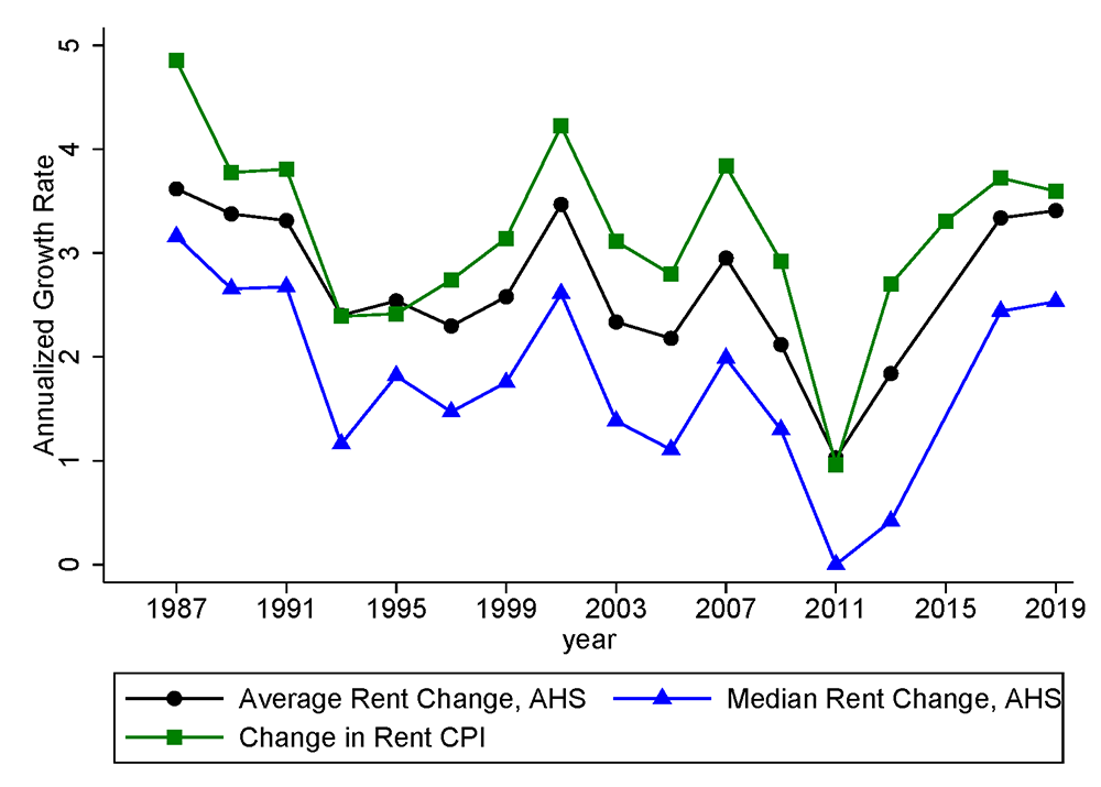
Note: The CPI is the published CPI for rent of primary residence.
Source: American Housing Survey, U.S. Census Bureau; Consumer Price Index, U.S. Bureau of Labor Statistics. https://www.census.gov/programs-surveys/ahs.html, https://www.bls.gov/cpi/.
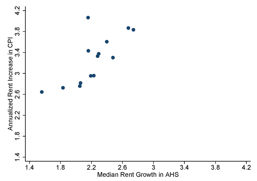
Note: Authors' calculations from the Consumer Price Index and the American Housing Survey. For the AHS, median rent growth was called for each metropolitan area and year, and the graph shows the average over all available years.
Source: American Housing Survey, U.S. Census Bureau; Consumer Price Index, U.S. Bureau of Labor Statistics. https://www.census.gov/programs-surveys/ahs.html, https://www.bls.gov/cpi/.
Figure 4 shows rent growth experiences in the AHS broken out by quintile of household income. We report median rent growth because the distribution of rent growth has a long upper tail, so average rent growth does not reflect the experience of most households in that quintile. In most years prior to 2003, rent growth was generally a little higher for the higher income groups, but this difference disappears in the second half of the sample. Table 2 reports that on average, the annualized rent growth rate for the fifth income quintile was 0.4 percentage points higher than the first quintile from 1985 to 2001. From 2001 to 2019, rent growth at the top was slightly lower than rent growth at the bottom. Cumulating over the entire 34-year period, rent rose by only 9 percentage points more for the top quintile than for the bottom quintile. Meanwhile, rent growth for the middle three quintiles was in between the growth rates for the top and bottom quintiles. Thus, on net the dispersion in rent growth across income groups was pretty minor over our sample period.
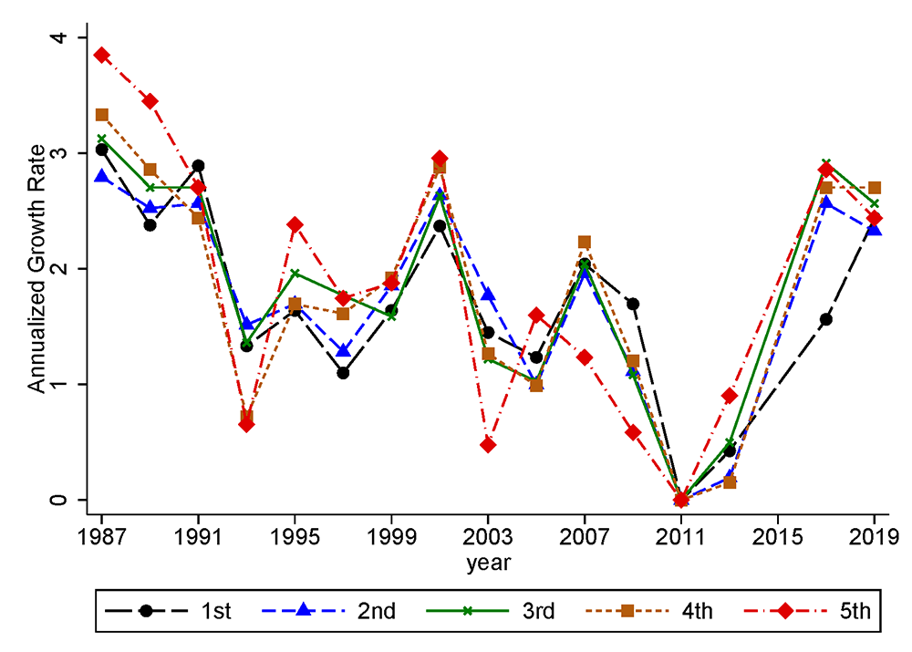
Note: Authors' calculations from the American Housing Survey. For growth rates from period t-1 to t, housing units are grouped by quintile of household income in period t-1.
Source: American Housing Survey, U.S. Census Bureau; https://www.census.gov/programs-surveys/ahs.html.
Table 2: Median Annualized Rent Growth by Income Quintile
| 1985-2001 | 2001-2019 | Cumulative Increase 1985-2019 | |
|---|---|---|---|
| Income quintile: | |||
| 1st | 2.01 | 1.41 | 72.40% |
| 2nd | 2.08 | 1.35 | 74.30% |
| 3rd | 2.17 | 1.31 | 79.20% |
| 4th | 2.17 | 1.38 | 77.60% |
| 5th | 2.44 | 1.23 | 81.20% |
Note: Authors’ calculations from the American Housing Survey. The cumulative increase reports the cumulation of the median 2-year changes, assuming no change in 2015 since changes cannot be calculated from 2013 to 2015.
Source: American Housing Survey, U.S. Census Bureau, https://www.census.gov/programs-surveys/ahs.html.
Implications for General Inflation by Income Quintile
We can create a general price index for each income group by assuming that the prices of all other goods and services purchased by households are the same across income groups. We use the Tornqvist price index formula below:
$$ (1) \ \ \ \ \ \ \ 1 + \pi^i_{t-1,t} = exp\bigg(\frac{s^i_{h,t-1}+s^i_{h,t}}{2} ln\big(\frac{p^i_{h,t}}{p^i_{h,t-1}}\big) + \frac{(1-s^i_{h,t-1})+(1-s^i_{h,t})}{2} ln\big(\frac{p_{xh,t}}{p_{xh,t-1}}\big) \bigg) $$
Where $$\pi^i_{t-1,t} $$ is the inflation rate for income group $$i$$ between time period $$t-1$$ and time $$t$$, $$s^i_{h,t}$$ is the housing expenditure share out of all household expenditures for income group $$i$$ in time $$t$$, $$p^i_{h,t}$$ is the price index for housing for income group $$i$$ in time $$t$$, and $$p_{xh,t}$$ is the price index for other goods and services in time $$t$$. For the price of housing services, we use an index created from the median rent growth rates of each income group. We calculate housing expenditure shares for each income group using data from the Consumer Expenditure Survey. In keeping with the CPI methodology, these expenditure shares are based on rental expenditures of renter households and the owners' estimate of the rent for their home for owner-occupied households. After calculating a housing expenditure share for each household, we take averages by year and income quintile. Figure 5 shows these expenditure shares. Lower income households spend a larger fraction of consumption on housing, and all households have spent a growing fraction of consumption on housing over time.
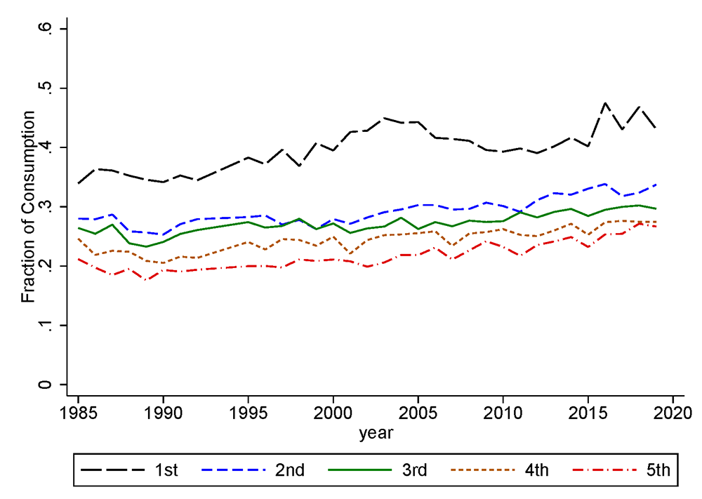
Note: Authors' calculations from the Consumer Expenditure Survey. Housing expenditures are rent for renter households and the owner's estimate of rent for owner-occupied households. The graph shows average housing expenditure shares for each income group.
Source: U.S. Bureau of Labor Statics, Consumer Expenditure Survey, http://www.bls.gov/cex/home.htm.
To implement equation 1 we also need an estimate of the non-housing price index. We calculate this index using the following data for all households as published as a part of the CPI program: the price indexes for tenants' rent, owners' equivalent rent of primary residence, and all items; and the expenditure shares for rent of primary residence and owners' equivalent rent of primary residence. We use the CPI index formula to back out the price index for non-housing goods and services.
One final issue to address is that we are using median rent growth to reflect the rent inflation experienced by each income group, whereas the CPI is designed to reflect average inflation experiences. Since median rent growth tends to be below the average (as we showed in Figure 2), simply using the medians for the price of housing services used in equation 1 would result in a general price index with lower growth than the CPI. We address this issue by calculating the difference between median rent growth in the AHS (across all income groups) and the growth rate of the CPI for tenants' rent for each two-year period. Then we add this difference to the median rent growth for each income quintile.8 Thus, the average rent inflation rate across income quintiles will be the same as in the CPI, while we preserve the differences across income groups calculated in the AHS.
Table 3 reports the general inflation estimates by household income group. In the first half of the sample, the estimates turn out to be quite similar across groups. Even though the higher income groups tended to experience higher rent growth, lower income groups tended to spend a larger fraction of their consumption on housing. Since rent growth even for the bottom quintile was faster than inflation for other goods and services, the higher consumption share for the bottom quintile boosts the general inflation rate for that group by more than the top income quintile. This effect turns out to roughly offset the higher rent growth faced by the higher income quintile during this period. In the second half of the period, the general inflation rate is a bit higher for lower income groups, owing to both their slightly faster rent growth and their higher share of housing services in consumption. Cumulating over the entire sample period, the differences across income groups are relatively small.
Table 3: General Annualized Inflation by Income Quintile
| 1985-2001 | 2001-2019 | Cumulative 1985-2019 | |
|---|---|---|---|
| Income quintile: | |||
| 1st | 3.12 | 2.43 | 143% |
| 2nd | 3.1 | 2.32 | 138% |
| 3rd | 3.13 | 2.31 | 139% |
| 4th | 3.11 | 2.28 | 137% |
| 5th | 3.14 | 2.23 | 136% |
Note: The general price indexes allow the price of housing services and the housing expenditure share to differ by income group. The price of non-housing goods and services is assumed to be the same across income groups. Authors’ calculations from the American Housing Survey, the Consumer Expenditure Survey and the Consumer Price index. The cumulative increase reports the cumulation of the 2-year changes, assuming no change in 2015 since changes in rent cannot be calculated from 2013 to 2015.
Source: American Housing Survey, U.S. Census Bureau; Consumer Expenditure Survey and Consumer Price Index, U.S. Bureau of Labor Statistics. https://www.census.gov/programs-surveys/ahs.html https://www.bls.gov/cpi/ , http://www.bls.gov/cex/home.htm.
An important caveat to this result is that inflation for non-housing goods and services could differ by income group. Research using scanner data, which mostly reflects retail goods like food, beverages, and housekeeping supplies, has found that inflation tended to be about 1 percentage point per year lower for the top income quintile than the bottom income quintile during the period 2004-2015 (Jaravel 2019, Kaplan and Schulhofer-Wohl 2017). These results suggest that inflation differences across income groups would be larger if other goods and services were taken into account.
Concluding thoughts
Differences in the price of housing services and the fraction of expenditures devoted to housing have not led to material differences in inflation across income groups over the past three decades. This result may be fairly surprising given prior research that has found substantial differences in housing costs in areas where high income households tend to live relative to areas where low income households tend to live (Moretti 2013; Gyourko, Mayer and Sinai 2013). It turns out that these geographic differences in housing costs overstate the rent growth differences faced by households in different income groups. One plausible explanation could be that lower income households are more likely to move out of areas with rising rents, bringing down average rent growth in areas where these households are observed living relative to the rent growth that we calculate absent this migration response. Also, households could sort differentially across neighborhoods within metropolitan areas in a way that reduces differences in rent growth across groups relative to the rent differences across metropolitan areas. Relatedly, rent growth tends to differ between single-family and multifamily units, even within the same neighborhood (Adams and Verbrugge 2021), which could lead to differences across income groups since higher income households are more likely to live in single-family homes. More research to understand why differential rent growth across metropolitan areas has not led to material differences in rent growth across the income distribution would be fruitful.
This article adds to the body of research that has investigated differences in prices paid or inflation rates faced by households across the income distribution (Argente and Lee 2020, Jaravel 2019, Kaplan and Schulhofer-Wohl 2017). However, the scanner data used in prior research accounts for only about 10 percent of the household consumption basket and rent accounts for an additional 25 to 30 percent, leaving more than half of the household consumption bundle for which differential inflation rates by income group have still been unexplored. More research should be done for these other types of household consumption to improve our understanding of how much and why inflation differs by income group.
References
Adams, Brian and Randal Verbrugge. 2021. "Location, Location, Structure Type: Rent Divergence within Neighborhoods" Federal Reserve Bank of Cleveland Working Paper 2103.
Garner, Thesia J. and Randal Verbrugge. 2009. "Reconciling User Costs and Rental Equivalence: Evidence from the US Consumer Expenditure Survey." Journal of Housing Economics 18: 172-192.
Gyourko, J., Mayer, C. and Sinai, T., 2013. Superstar cities. American Economic Journal: Economic Policy, 5(4), pp.167-99.
Heston, Alan and Alice O. Nakamura. 2009. "Questions about the Equivalence of Market Rents and User Costs for Owner Occupied Housing." Journal of Housing Economics 18: 273-279.
Jaravel, Xavier. 2019. "The Unequal Gains from Product Innovations: Evidence from the US Retail Sector" Quarterly Journal of Economics 715-783.
Kaplan, Greg and Sam Schulhofer-Wohl. 2017. "Inflation at the Household Level" Journal of Monetary Economics 91: 19-38.
Moretti, Enrico. 2013. "Real Wage Inequality" American Economic Journal: Applied Economics 5(1): 65-103.
Semega, Jessica, Melissa Kollar, Emily A. Shrider and John F. Creamer. 2020. "Income and Poverty in the United States: 2019". Current Population Reports, US Census Bureau.
* The analysis and conclusions set forth are those of the authors and do not indicate concurrence by other members of the research staff or the Board of Governors. Return to text
1. Specifically, rent is used to calculate changes in the price of housing services faced by both renters and owner-occupants. Return to text
2. The purchase price of a home reflects the price to invest in housing, not the price of housing services. Similarly, owner expenditures such as mortgage and property tax payments reflect the price of owning the asset, not the price of consuming housing services. Although the user cost of owning a home should equal the price of housing services in theory, in practice some components of the user cost are difficult to measure. Return to text
3. Rent is topcoded at about the 97th percentile in each year. For 1997 and later years, the topcode is equal to the average rent among topcoded observations. For earlier years, the topcode is equal to the 97th percentile. To make the early years consistent with the later years, we multiply the pre-1997 topcode value by 1.5, since the post-1997 topcode values are roughly 50 percent higher than the rent at the 97th percentile. Return to text
4. Specifically, we regress the natural logarithm of rent on year indicators, the housing characteristics, and the indicators for metropolitan area. We calculate the residual from this regression, adding back in the estimated coefficients on the year indicators. The table reports the percent change in the average residual by income group. Return to text
5. There is no indicator for renovation prior post-2013. We also drop imputed rent values. Return to text
6. These cutoffs are an annualized log change of -0.21 at the bottom and 0.29 at the top. Return to text
7. This gap diminishes if we do not trim the top and bottom 5 percent of rent changes, but without the trimming average rent growth is extremely volatile year to year. Return to text
8. This difference is about 1 percentage point, on average. Return to text
Larsen, Daryl, and Raven Molloy (2021). "Differences in Rent Growth by Income 1985-2019 and Implications for Real Income Inequality," FEDS Notes. Washington: Board of Governors of the Federal Reserve System, November 05, 2021, https://doi.org/10.17016/2380-7172.3006.
Disclaimer: FEDS Notes are articles in which Board staff offer their own views and present analysis on a range of topics in economics and finance. These articles are shorter and less technically oriented than FEDS Working Papers and IFDP papers.