FEDS Notes
July 01, 2022
An Approach to Quantifying Operational Resilience Concepts
Chase Englund and Carlos Sosa1
I – Introduction
In the years following the global financial crisis, the international regulatory community implemented a number of measures aimed at reforming the global prudential framework and enhancing the stability of the financial sector. The resulting structural changes have improved the financial resilience of firms through stronger capital requirements, liquidity buffers, and enhanced recovery and resolution mechanisms to lessen the impact of a firm's financial failure.
Yet, despite a safer system that is more resilient to financial vulnerabilities, efforts to safeguard the financial system against operational failures and disruptions arising from events such as cyber-attacks, pandemic outbreaks, natural disasters or terrorist attacks are still being developed. Large-scale shocks such as these have either already occurred or appear increasingly likely, and thus it seems plausible to suspect that events such as these will eventually result in significant operational failures or disruptions that will test the financial system's recent financial resilience gains.
In recent years, regulatory authorities and international standards setting bodies have begun to develop approaches for operational resilience. Among these was SR 20-24, Sound Practices to Strengthen Operational Resilience. These efforts continue to develop. Importantly, these efforts have highlighted how operational risk could plausibly result in systemic-level disruptions to critical operations and core business lines. The Federal Reserve's 2021 Financial Stability Report cited operational risks related to cybersecurity, especially those involving the impairment of or access to major payment systems, as a top financial stability concern for 2021. While different from a "traditional" financial crisis, these shocks could plausibly generate similar destabilizing outcomes, particularly when shocks are large enough to trigger significant second-order financial consequences and loss of confidence in financial markets. According to an independent study commissioned by the ECB, in May 2020, an operational failure of the TARGET2 Securities clearing system resulted in over 740,000 transactions being halted for approximately 12 hours (ECB 2021), representing a daily disruption value of over 1 trillion euros (ECB 2020).
This work uses publicly available data to demonstrate how concepts from recent guidance and a variety of academic literature on operational resilience and operational risk events can be used to construct a basic methodology for creating a map of operational interconnectedness, simulating disruptions to such networks, and estimating the operational impact of these disruptions. While by no means definitive or all-encompassing, the methods demonstrated here provide a starting point for conceptualizing some of the regulatory concepts contained in guidance like SR 20-24, which covers a topic area of rapidly growing importance. The estimates generated by this paper are intended to provide an illustration of how operational resilience concepts can be quantified and used to inform decision making around risk mitigation measures and the setting of tolerance thresholds.
II – Context and Past Research
Recent literature has demonstrated a number of linkages between operational risks, particularly cyber risk, and financial stability (see for example Boer and Vasquez, 2017, Kopp, Kaffenberger, Wilson, 2017, Warren, Kaivanto, and Prince, 2018, among many others). Along these lines, there have been a number of efforts aimed at examining financial losses due to operational risk events. These studies provide important insight into how operational risk effects firms' financial resilience and how such impacts can present financial stability concerns (see for example Berger et al. 2020, or Curti, Migueis, & Stewart 2019). Research and models that predict or estimate financial losses from operational risk form the basis of the Advanced Measurement Approach (AMA) and the Standardized Approach (SA) utilized by the Basel Committee on Banking Supervision.
Less studied than financial resilience is how such events impact operational resilience. This key difference has important ramifications. While the risk of financial loss can have significant consequences for financial stability, events in which operational disruptions impact large volumes of financial-sector activity (which could be financial flows or other activity like dataflow), even temporarily, can also have significant impacts on systemic stability. Even when operations are resumed and the direct financial loss to the involved firms is relatively small, the impact that such disruptions can have while they are ongoing (and sometimes after) is often magnitudes larger than the direct loss impact. A number of recent studies have attempted to examine the direct and indirect impacts stemming from operational risk events (for example Eisenbach, Kovner & Lee 2020, or Crosignani, Macchiavelli, and Silva 2021).
The Federal Reserve's SR 20-24, Sound Practices to Strengthen Operational Resilience, defines operational resilience as "the ability to deliver operations, including critical operations and core business lines, through a disruption from any hazard". Along these same lines, the concept of operational resilience has most commonly been defined in the scientific literature as a measure of the ability of a complex system to withstand and recover from disruption events2 to continue functioning as intended (see for example Essuman, Boso, and Annan 2020, Ganin et al. 2016, or Ros & Schaanning 2020). Essuman, Boso, and Annan (2020) refer to this conceptualization of operational resilience as "output-base resilience". By determining what the base level of "critical functionality" is for a complex system, we can quantify how resilient that system is by measuring the degree to which a disruption reduces that critical functionality, and how quickly the system recovers from that reduction (Ganin et al. 2016).
In order to measure resilience, we must also define and quantitatively measure the concept of disruption itself. Disruption refers to an interruption in the ability to deliver functionality as a result of the manifestation of some operational risk (such as a natural disaster, cyber-attack, etc.). For the critical operations and core business lines of the financial sector, functionality is typically measured in dollars. Alderson, Brown, and Carlyle (2015) conceptualize disruption as a level of "cost" to system functionality associated with "attacks" of various severity. In their models, the severity of the event is causal to the corresponding level of disruption experienced by the system. They also incorporate "mitigation strategies", which are changes to the network (either creating new links or strengthening existing links) designed to improve resilience. The effectiveness of these strategies is assessed by measuring their impact to disruption size and resilience at each level of event severity.
This conceptualization of disruption is useful in that it provides a means by which we can define and measure disruption to financial operations. The "product" that the financial system delivers is measured in units of currency, and therefore any quantification of disruption must use units of currency as its measure to determine the severity of an operational disruption. Similar to the Alderson, Brown, and Carlyle (2015) models, we can sketch disruption size3 as a function of the level of operational risk event severity (i.e. the number of impacted nodes in a network) as a basis for determining when an event can be suspected to have systemic ramifications, and also as a way of evaluating mitigation strategies.
Existing bank regulation and guidance has also established the concept of "tolerance for disruption". SR 20-24 defines this term as "a firm's risk appetite for weathering disruption from operational risks…informed by existing regulations and guidance [such as SR 03-9, Interagency White Paper on Sound Practices to Strengthen the Resilience of the U.S. Financial System]". SR 03-9 states that "firms that play significant roles should plan to recover clearing and settlement activities…within the business day on which a disruption occurs". By quantifying the disruption size that a breach of this same-day tolerance by several large banks (subject to supervision by the Large Institution Supervision Coordinating Committee, known as LISCC) would entail at various levels of operational disruption, we can examine at what point such an event could be expected to have consequences for overall financial stability.
One example of this concept in application is found in Ros & Schaanning (2020). The authors develop a conceptual model of how one type of operational risk, a cyber-attack, can develop into a systemic event for the financial system. They describe a concept similar to that of tolerance for disruption, and present a framework in which events of varying severity and duration become systemic at varying points. A primary takeaway from their framework is that an operational risk event in which the disruption size ("aggregate impact") exceeds a certain threshold of severity and duration can be expected to have financial stability concerns.
Another recent example of this concept is found in Eisenbach, Kovner and Lee (2020). The authors examine a hypothetical cyber-attack that disconnects targeted firms from the Fedwire Funds Service. They use data on intraday payments between banks in the Fedwire Funds Service payment system to estimate the size of the resulting disruption, and further estimate which firms would drop below their average liquidity "impairment threshold" as a result of the event. They estimate that 60% of firms within that payment network would become impaired in the event of the hypothetical scenario they describe. The Fedwire Funds Service payment system services several trillion in transactions per day, and they estimate that a total disruption to service for one of the top five payment system users would result in a disruption size several times larger than US daily GDP. While this work provides a rich exploration of one hypothetical disruption event, it can be expanded by introducing conceptualizations of overall resilience, duration and recovery, tolerance for disruption, and mitigation.
Another recent study that shares a similar premise is found in Kotidis & Schreft (2022). Instead of hypothesizing a disruption event, this paper uses data from an actual cyber event that caused the outage of a third-party software that firms used to send Fedwire payments. They quantify part of the operational impact on banks by measuring Fedwire payments among banks that used the service in comparison with those that did not. Their work finds that firms impacted by the outage sent as many as 36% fewer payments through Fedwire on the first day of the incident, and 16% fewer payments on average through the duration of the incident. This study is important because it provides an actual example of an operational disruption caused by an operational risk event, and attempts to quantify the resulting disruption. By estimating a regression coefficient for the reduction in payment activity statistically attributable to this particular cyber event, it provides a plausible estimate of how resilient firms might be to a critical service outage. The concepts developed by this study, as well as by Eisenbach, Kovner and Lee (2020) can be used to help quantify concepts such as resilience, duration and recovery, tolerance for disruption, and mitigation.
While much of this groundbreaking work focuses on operational disruptions to payment systems related to cyber-attacks, it is also important to note that operational risks are varied, with cyber-attacks representing just one of many potential scenarios that may cause an interruption in the operation of critical operations and core business lines. Furthermore, payment, clearing and settlement is only one of numerous of these critical operations and core business lines, which are also varied and include functions related to consumer and commercial banking, funding and liquidity, capital markets, and custody and safekeeping.
III – Data
Section 165(d) of the Dodd-Frank Wall Street Reform and Consumer Protection Act requires that bank holding companies with total consolidated assets of $50 billion or more periodically submit resolution plans to the Federal Reserve and the Federal Deposit Insurance Corporation. Each plan, commonly known as a living will, describes the company's strategy for rapid and orderly resolution in the event of material financial distress or failure of the company, and include both public and confidential sections.
The resolution plans contain data on each firm's material entities, financial market utility (FMU) memberships, and financial condition. Currently, the largest, most complex banking organizations supervised by the Board are required to file resolution plans by July 1 of every other year. The data used for this model was collected entirely from the July 2021 filing for each of the eight LISCC-designated banks.4 The data on firms' FMU memberships is utilized to develop a proxy network map of firms' operational dependencies on these entities, which serve as critical service providers to these firms' critical operations and core business lines. A rendering of the sample network is shown in Figure 1 below. The figure contains the eight LISCC banks and 60 unique FMUs reported in the resolution plans.
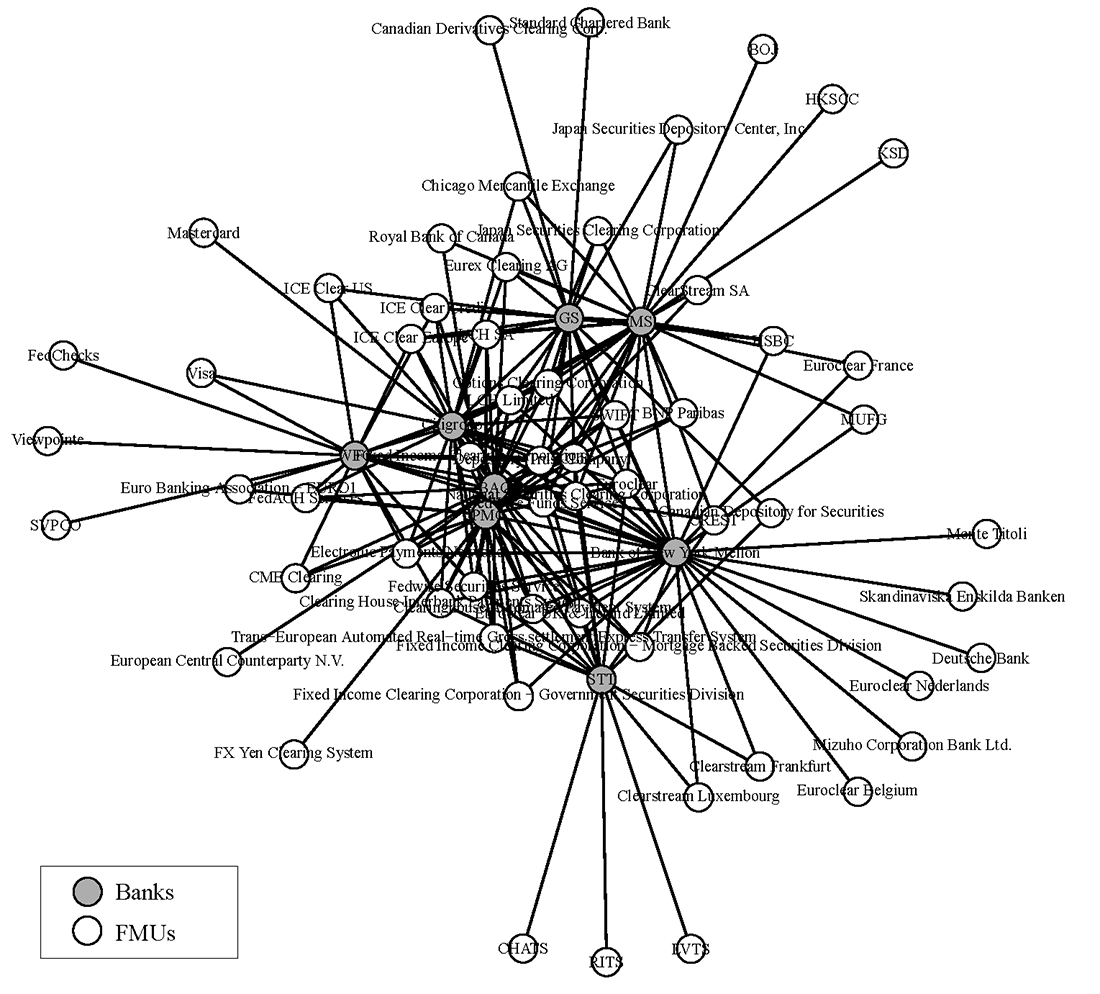
Financial Market Utilities are often important participants in a number of bank critical operations and core business lines. The FMUs reported in the public resolution plan filings are entities related to payment, clearing, and settlement (PCS), although FMUs also exist and function in a number of other critical operations and core business lines outside of PCS. The data here should be considered a limited sample that provides an approximation of FMU exposure related to one type of critical operation (PCS).
The National Information Center, maintained by the Federal Financial Institutions Examination Council (FFIEC), contains a repository of financial data and institution characteristics collected by the Federal Reserve System. Much of this data is available for general public access. Among this public information is the Systemic Risk Report FR Y-15 snapshots, which provide data from individual firms' FR Y-15 submissions. The FR Y-15 contains firm-specific data on a number of risk exposure variables. Among these is yearly-aggregate overall payments activity. While not a perfect measure, we can use this figure to generate a proxy estimate of a bank's daily operational exposure to key payment systems. While this does not allow for an approximation of the size of operational exposure to all FMU entities in the network, it is applied to the payment-focused entities.
Figure 2 provides a rendering of the network with only the payment system FMUs listed. The connections depicted here should not be considered a complete picture of payment system operational interdependence, but rather a simplified representation. Firms typically rely upon third party service providers to interact with these payment system FMUs, and these relationships are not depicted in this simplified image. Furthermore, the relationships shown here are only the key relationships that are reported by the firm in their public filing. Each firm may, and likely does, have some form of relationship with each of the payment FMUs listed here. However, connections are only shown where the firm reported the relationship in their public filing, ostensibly because the relationship was deemed operationally significant enough to report. For the purposes of this exercise, every LISCC firm was assumed to have an operationally significant relationship with the Fedwire Funds Service, although (perhaps surprisingly) not every firm reported this connection.
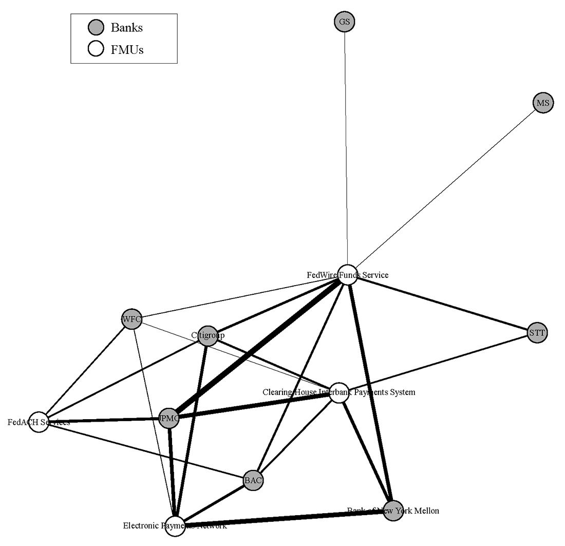
The Clearing House Interbank Payments System (CHIPS) is a United States private clearing house for large-value transactions. Together with the Fedwire Funds Service (which is operated by the Federal Reserve Banks), CHIPS forms the primary U.S. network for large-value domestic and international USD payments where it has a market share of approximately 96%. For payments that are less time-sensitive in nature, banks typically prefer to use CHIPS instead of Fedwire, as CHIPS is less expensive (both by charges and by funds required). One of the reasons is that Fedwire is a real-time gross settlement system, while CHIPS allows payments to be netted.
The Electronic Payments Network (EPN) is an electronic clearing house that provides functions similar to those provided by Federal Reserve banks. The Electronic Payments Network is the only private-sector operator in the ACH Network in the United States. FedACH is the Federal Reserve Banks' automated clearing house (ACH) service. In 2007, FedACH processed about 37 million transactions per day with an average aggregate value of about $58 billion. For comparison, Fedwire processed about 537,000 transactions per day valued at nearly $2.7 trillion in the same year.
Figure 2 provides information about the interconnectedness of the eight LISCC banks and these four payment FMUs. The estimated volume of payments is indicated by the thickness of the line linking each part of the network (known as "edge weightings"). The edge weightings are derived from the previously described Y-15 data. The methodology used to assign the edge weight values is described in more detail in Section V. It is important to note that no data on connections between the banks themselves is modeled, as this information is not reported in the source data. The data shows the connections of each bank with the various FMU entities chosen for this simulation.
IV – Model
The model used within this analysis relies partly on each firm's position within the FMU network. By hypothesizing disruptions to certain nodes within the network, we can use the network map to trace the impact of such events and generate estimates of disruption to the financial system, as well as the overall resilience of the system. This analysis is also taken a step further by incorporating elements of time, as well as node position within the network to condition these cost and resilience variables.
Disruption is conceptualized in a manner similar to what is described in Eisenbach, Kovner and Lee (2020), where disruption is essentially defined as the quantity of normal business transactions foregone, delayed, or cancelled as a result of an operational disruption.
The size of this disruption will be some function of firms' exposure to the event, the severity of the event itself, and the level of mitigation employed by the firm. I utilize a model of disruption in dollars stemming from a disruption event which is specified here as:
$$d = f (n, e, m)$$
Where $$d$$ is the size of the operational disruption measured in dollars, $$n$$ is a measure of the firms’ relative exposure to the event, $$e$$ is the severity of the disruption event, and $$m$$ is the level of mitigation steps applied pre-event, relative to the base case.
In the models estimated here, disruption events are hypothesized as equally impacting each of the eight LISCC banks' ability to interact with a specific FMU simultaneously. Multiple banks can lose access to an FMU simultaneously if they are utilizing the same third-party service provider to interact with that FMU. If that service provider is affected by a disruption that interrupts functionality (such as a cyber-attack), multiple clients can be affected simultaneously. Additionally, a disruption that originates at the FMU itself may also result in this type of simultaneous impact (although this would have an impact beyond the connections modeled here). This simplifying assumption of the model (simultaneous disruption of interaction with a particular FMU) is useful here, as the data contains information on banks connections with FMUs, but not necessarily with each other. In reality, an operational disruption could impact banks FMU connections heterogeneously (some banks lose access to an FMU, while others do not), and may also impact banks direct connections with one another (these connections are not estimated here). While the network data does contain information about linkages between the LISCC banks and other agent banks, the volumetric data we employ to estimate connection size applies specifically to payments, so our estimations are contained to payment system FMUs and connected banks.
A firm's exposure to the event is quantified by virtue of its position within the network. The greater the 'size' of the event (i.e. the number of impacted nodes and the higher the value of their linkages), the greater the exposure. The severity of the event is some expected reduction in activity measured as a proportion of the firms' link-specific operational exposure to the FMU.
Mitigation is quantified as some reduction in a firms' expected impact severity from the baseline, either by virtue of better operational resilience practices around existing links, or through the procurement of substitute links to 'work around' disruptions. The level of mitigation present can be thought of as a function of firm preference, regulatory requirement, or both. In the application here, variation in mitigation is applied uniformly across firms, but a firm-variable (i.e. heterogeneous) approach would also make sense.
By visually displaying the estimated size of an operational disruption as a function of these variables, we can assess the appropriateness of various mitigation options and the likelihood that an event will carry systemic impact, similar to the methods employed by Alderson, Brown, and Carlyle (2015) or Ros & Schaanning (2020).
Following suit with concepts developed in Ganin et al. 2016 and Essuman, Boso, and Annan 2020, resilience is conceived as the degree of critical functionality retained by the network following a disruption. This measure, System Resilience $$(R)$$ is conceived here as a measure between 0 and 1, or 0 and 100, indicating the percentage of nodes within the network that are still operational multiplied by their associated network value. We can define our measure of resilience using the following specification:
$$R=$$ (Value of Active Functionality) / (Value of Total Functionality)
It is important to note that the value of this measure will be conditioned by the size of the network. In other words, a network with fewer, more valuable nodes will lose resilience more quickly than a larger network that incorporates a more wholistic picture of the market. One potential way to account for this factor is to estimate a network completeness value alongside the System Resilience value. A network completeness value is a measure of the difference between a network depiction and the real-world network in terms of output. This difference comes from nodes being excluded from the depiction due to missing data, simplification, or some other reason. This value allows the analyst to discount the resilience measure accordingly. For example, where the estimated completeness of a network is 0.5, roughly half the critical functionality of the real-world network is excluded from the sample estimate. This will result in a measure of resilience that is likely lower than the true population value with the excluded nodes included.
As discussed, most conceptualizations also include some incorporation of time into the estimate (for example Ganin et al. 2016, or Ros & Schaanning 2020). This accounts for the fact that the size of a disruption will increase concurrently with the duration of a disruption, and also for the fact that firms may recover some functionality before an operational disruption event ends completely.
To incorporate a time measure, each variable (disruption size, resilience) becomes a summation across all values of $$(t)$$, discounted by the measure of recovery $$(r)$$. For example, for disruption size we specify:
$$$$ \sum_{t=1}^n (d * r) $$$$
In this estimate, $$(t)$$ is equal to the total time multiplier, a function of the number of hours for which a disruption endures.5 Other models may use other measures, such as days, or other factors, such as the time the disruption event began, to illustrate greater heterogeneity over various thresholds. For example, an event that begins in the afternoon and extends for eight hours may be exponentially more disruptive than an event that begins in the morning and lasts for four hours. The second value, recovery, can be estimated at the network-level, but is also applicable to the firm-level, as firms may differ in their ability to recover. In this way, the recovery variable is similar to the previously discussed mitigation measure used to estimate disruption size.
V – Model Application
In order to proxy the operational exposure of the payment system FMU links, each firm's average total daily payments exposure was divided across the payment system FMU memberships it displayed in the network. By this measure, when comparing two banks with the same level of payments exposure, the bank with fewer payment system FMU links would have a higher exposure value for each link (a proxy measure for its lower capacity to utilize substitute services in the event of an outage).
One way to estimate connection volumes is to assume that each FMU channel is equally utilized. However, in reality some providers are likely to facilitate more volume than others. To approximate this variation, the estimation of exposure values applied here uses weighting to distribute the volume. The estimation is found by taking the total exposure value for a bank node divided by the total number of linkages for each connected payment system FMU, yeilding a constant for each bank. The value for each of that bank's linkages is found when this constant value is multiplied by the number of linkages attributed to the corresponding FMU entity. With this method, the estimated volume between a bank and an FMU is weighted by how many other banks are connected with that particular FMU in the model. FMUs with more connections are assumed to have more volume.
A simple example helps illustrate each estimation method. Suppose Bank A has two payment system FMU connections. The first FMU (FMU 1) hosts two other banks, while the second FMU (FMU 2) has only Bank A as a client. To find the constant for Bank A, the bank's total exposure is divided by four, which is the total number of linkages attributed to the FMU entities connected to Bank A (FMU 1 has three connections, and FMU 2 has one connection). Each linkage value for Bank A is then determined by multiplying this constant by the corresponding number of FMU connections. So the estimated link value between Bank A and FMU 2 is the total exposure divided by four and then multipied by three, and the estimated link value between Bank A and FMU 1 is the total exposure divided by four and then multipied by one. The weightings for each FMU in this model can be found in the solutions appendix. The weightings roughly correspond with the Eigenvector Centrality score for each of the FMUs (also found in the appendix), meaning that this measure could also serve as a suitable weighting value for more complex networks.
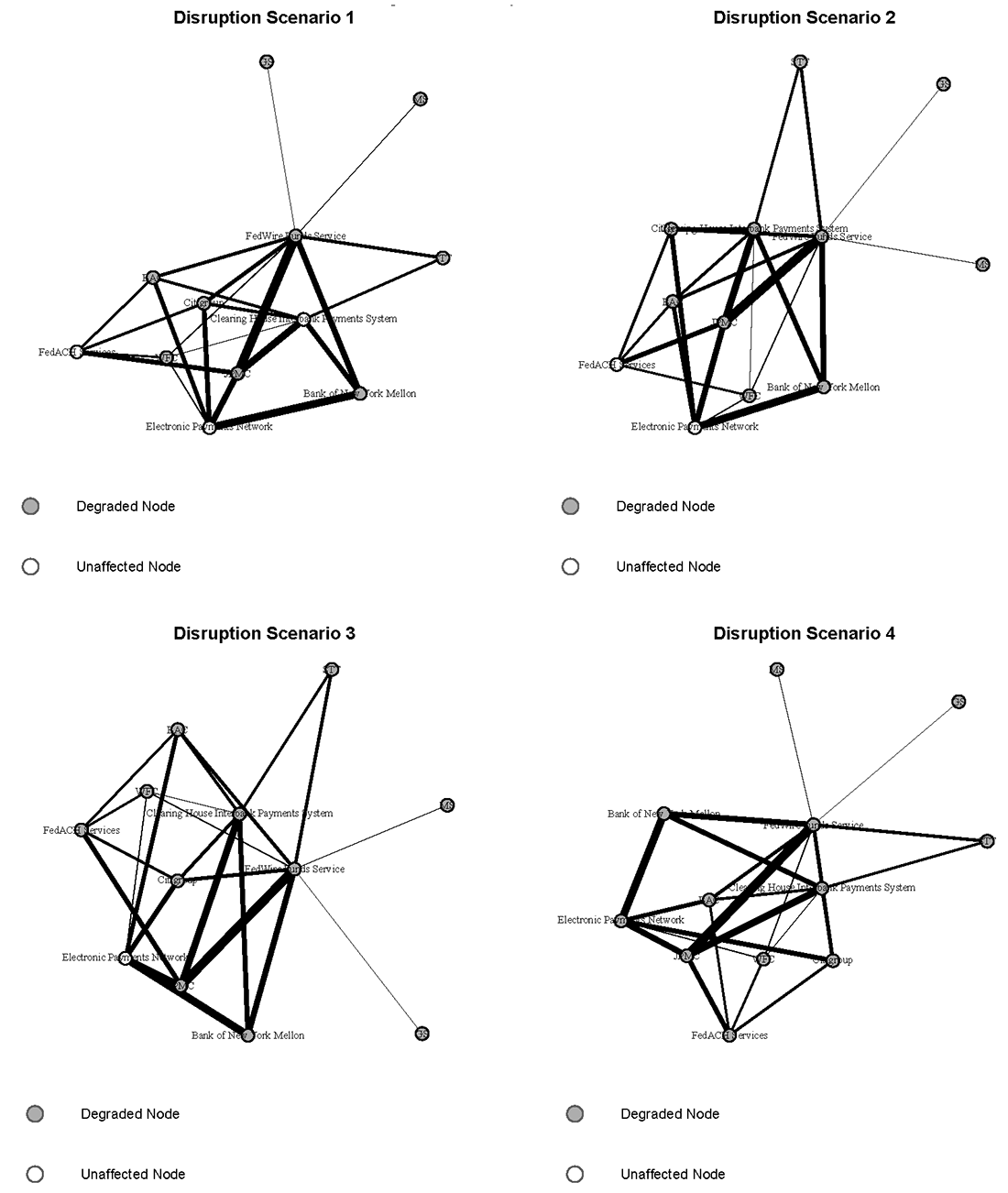
To construct a measure of disruption size at varied levels of disruption event severity, four disruption scenarios are hypothesized, in which the number of disrupted payment FMU entities increases sequentially. These events are hypothetical, and can be thought of as having variable probability, with event severity being negatively correlated with probability of occurance. The application here does not assume probability values, as these are intended primarily to be illustrative models.
The value for disruption size was calculated by multiplying the exposure value for each link by a constant value. This constant, the 'disruption coefficient', was set at a baseline of 0.5, following an approximate "first-day" benchmark found in Kotidis & Schreft (2022).6 This baseline constant was then adjusted to simulate various levels of "mitigation". Mitigation represents efforts by a firm to become more operationally resilient. By employing various practices7 to enhance operational resilience, firms can better sustain operational disruptions and employ alternative channels to continue functioning.
At Mitigation Level 1, the constant was adjusted down by 0.1 (resulting in a disruption coefficient of 0.4), and at Mitigation Level 2, the constant was adjusted down by 0.2 (resulting in a disruption coefficient of 0.3). Second-day disruption size was estimated at 0.25 times the exposure value, using the same approximate standard deviation to adjust for mitigation (0.1), following the assumption that attacked firms regain some capacity to transact as time goes on. This is consistent with the finding from Kotidis & Schreft (2022), similar to the coefficient they found for the overall average reduction in activity (as opposed to "first-day").8
An illustration of the various disruption scenarios can be found in Figure 3. In Disruption Scenario 1, the firms' connections with the Fedwire Funds Service are disrupted. As the figure illustrates, the size of the impact from this disruption for each firm depends on the payments volume of that firm with Fedwire. However, for most of these entities, alternative same day payment channels exist through significant reported relationships with CHIPS, as well as ACH options through FedACH or EPN. Having payment exposure spread out across more linkages results in a lower impact from the degregation of one such linkage. In Scenario 2, the banks' connections with both critical USD same day payment channel, CHIPS and Fedwire, are impacted. In Scenario 3, the disruption is expanded to include both same day payment channels and the FedACH system. In Scenario 4, the most severe scenario, the disruption impacts firms' ability to interact with any of the key reported USD payment system FMUs.
By estimating these disruption events of varying severity, and also estimating various levels of assumed mitigation, we can use the estimated values associated with each FMU link to sketch approximations of both how large the hypothesized disruption would be, and the resulting level of resilience for each scenario.
The first of these curves can be seen in Figure 4, which depicts the disruption size $$(d)$$ resulting from each scenario. For an example solution for $$(d)$$, reference the appendix. As the figure illustrates, increasing event severity results in an increasingly large disruption. Increasing levels of mitigation results in lower levels of disruption, shifting the disruption curve downward. From a theoretical standpoint, the beginning and end points of each curve should move towards convergence. While not illustrated, a scenario in which there is no disruption would have all three curves converged at zero, while a disruption so severe that no mitigation strategy was effective would see all three curves converge at some greater level of disruption. With no mitigation, the estimated disruption from the most severe scenario was approximately 1.4 trillion USD.
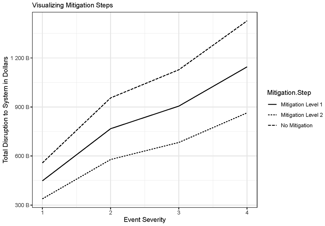
Figure 5 depicts the overall level of resilience $$(R)$$ in the model resulting from each scenario. For an example solution for $$(R)$$, reference the appendix. As the figure illustrates, increasing event severity (Disruption Scenario 1 being the least severe, and Disruption Scenario 4 being the most severe) results in decreasing levels of resilience. Increasing levels of mitigation result in higher levels of resilience, shifting the resilience curve upward. From a theoretical standpoint, the beginning and end points of each curve should move towards convergence. While not illustrated, a scenario in which there is no disruption would have all three curves converged at 100% resilience, while a disruption so severe that no mitigation strategy was effective would see all three curves converge at some lower level of resilience. With no mitigation, the estimated disruption from the most severe scenario resulted in a resilience level of roughly 50%, reflecting our assumed disruption coefficient being applied to every link.
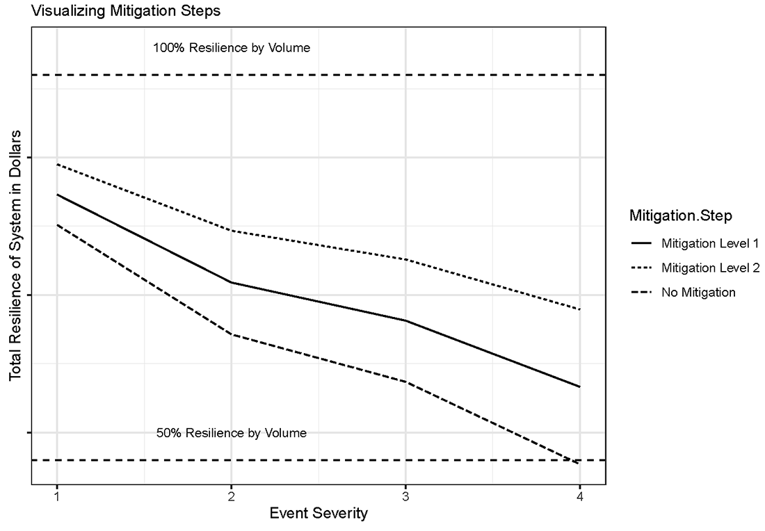
The values shown in Figures 4 and 5 were found by utilizing the weighted method for estimating linkage values discussed at the beginning of this section. The curves illustrated in both Figure 4 and Figure 5 are static, meaning that they do not account for temporal variation. By incorporating a measure of time $$(t)$$, we can improve our understanding of the practical implications of a disruption event.
The chosen unit of $$(t)$$ in this case was hours. Figure 6 provides an illustration of resilience over a theoretical window of time for which the disruption event continues. As an event continues, firms are able to adjust their operations to work around the disruption. This concept, known here as recovery, has a mitigating effect on the disruption over time. We assume that firms recover roughly 50% of their capacity to continue operations after the first day of an event. For illustrative purposes, Figure 6 assumes that recovery begins after hour 14. No ending time is hypothesized for the event, but the model assumes that firms will continue to operate at the recovered value ($$R^R$$, or 0.25) until the disruption event ends (at some point past hour 25 in this case). The curve shown in Figure 6 could be duplicated for the various levels of disruption and mitigation hypothesized by the model.
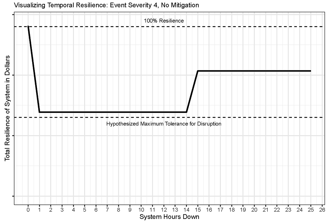
Figure 6 also includes a line depicting the "Hypothesized Maximum Tolerance for Disruption",9 which is shown at roughly 49% resilience. This indicates a threshold at which the level of resilience would be considered unacceptable, either due to financial stability concerns or some other criteria. The threshold shown here is only for illustrative purposes, but in a model where an actual Tolerance for Disruption was defined, a breach of that threshold would represent the need for additional mitigation.
While Figure 6 provides a useful illustration of resilience over time, it is not sufficient to fully understand temporal variation across a disruption event. Low resilience (50% in this case) for a short period of time will be inherently less disruptive than low resilience for a longer period of time. In order to illustrate this concept, we sketch a temporal curve for disruption size, shown in Figure 7. The true impact of an event would be a function of both time and the time of day during which the event began (an event that starts earlier in the day can last longer before becoming a multiday event). In this case we assume that an outage of over 11 hours crosses the threshold from a same-day event to a multiple-day event. For a same day event, the disruption multiplier is assumed to be zero. When a disruption is resolved before the end of the same-day window, transactions can still be completed, and the normal flow of financial activity is not materially disrupted. Once this window is breached, the disruption size will multiply by the number of business days for which it continues. Using days as the unit of time measurement is appropriate here because our disruption curves were sketched using daily terms.
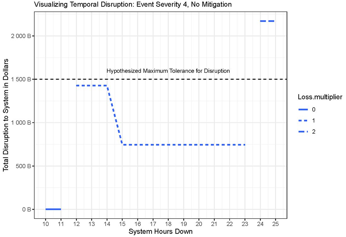
Figure 7 is useful for several reasons. First, it provides a more realistic way to determine whether an event will exceed an acceptable level of disruption. As the figure demonstrates, when the Hypothesized Maximum Tolerance for Disruption from Figure 6 is converted into a dollar figure for Figure 7, the level of disruption actually exceeds the maximum tolerance when the event continues into a second day (shown here for illustrative purposes as occurring at hour 24), even after recovery begins at hour 14. This approach allows an analyst to utilize the model to determine a maximum tolerance for disruption, and express this tolerance either as a dollar figure (in this case 1.5 trillion USD) or a specific number of hours (in this case is 24). Insofar as existing regulatory thresholds are expressed in either of these terms, a model such as this allows an analyst to convert a threshold from one form to the other.
The various measures of tolerance for disruption can also be used in combination. For example, Figure 7 implies a maximum tolerance for disruption of 24 hours (these time-based measures can also be thought of a total "recovery time objectives"). However, this figure was arrived at by assuming that the system would maintain at least 50% resilience, or less than 1.5 billion USD in halted transactions, during the disruption. Therefore, we might say that our desired maximum tolerance for disruption is a loss of no more than 50% resilience with a total recovery time objective of 2 days.
For a number of reasons, a resilience-based maximum tolerance for disruption (i.e. 50% in this case) may be preferred over a limit expressed in dollars when setting guidelines. Once we find the time variant disruption size in actual dollars and determine the desired limit, we can also adjust resilience thresholds with some length of time in mind. For example, if we wish to set a total recovery time objective of three days instead of two, the minimum level of resilience maintained during the event must be some percentage greater than 50%.
These methods are potentially useful for framing a discussion about operational resilience and financial stability. The most severe disruption event hypothesized by this model, Scenario 4 with no mitigation, entails a static disruption size of roughly 1.4 trillion USD per day before recovery, and roughly 700 billion per day after recovery begins. This value is enough to plausibly constitute some risk to overall financial stability by itself, and it is clear that a disruption of this nature which lasted for a long enough period would significantly exacerbate this risk. This highlights the importance of measures to ensure resilience within certain timeframes, and the potential usefulness of models such as this in examining such standards.10
It should also be noted that this estimation is only providing an illustration of first order effects. Second (and third) order effects would likely amplify the size of the disruption estimated here by several times (see Diebold & Yilmaz 2015 or Schreft & Zhang 2018 for further discussion of transmission).
VI – Conclusion
With knowledge of the proper variables and an understanding of how a particular critical market is organized, a model such as the one illustrated here allows for practitioners to anticipate the damage from various types and levels of disruption event, as well as test the viability of various mitigation strategies. It also provides a quantitative language with which to describe concepts like operational disruption, operational resilience, recovery, and tolerance for disruption. Lastly, it provides a way to convert static measures into temporal curves, which allow analysts to consider the implications of existing tolerance thresholds and, if appropriate, select new ones.
While this model does not seek to prescribe any specific policy measures, it is plausible that methods similar to those shown here could assist in developing such measures in the future. Methods such as these, which are designed to quantify operational disruption, will be important tools to analyze what policy responses (both public and private) are appropriate to various operational risks. Specifically, methods such as this can help estimate the level at which operational disruptions can develop from serious, but ultimately contained events, into systemic events where the disruption is severe enough to harm confidence in the financial system and create significant damage in the real economy. What happens after the breach of a tolerance for disruption is a question for both firms and regulators that deserves further discussion and analysis. Such an occurrence could conceivably be a trigger for specific actions by the firm or regulators to contain an event.
While the data employed here is somewhat limited, the conceptual model demonstrated is transportable. The purpose of this work is to illustrate one way in which common operational resilience lexicon and concepts can be employed in a straightforward quantitative analysis, and how such analysis can inform decisions around risk mitigation and setting tolerance thresholds. More data, both on operational interconnectedness and on the impacts of operational risk events, would serve to make analysis like this more realistic and useful. As better data becomes available, techniques and concepts similar to those employed here offer a tangible way in which policy makers, academics, and industry practitioners can standardize the discussion of operational resilience and develop data-driven standards.
References
- Acemoglu, D., Ozdaglar, A., & Tahbaz-Salehi, A. (2015). Systemic risk and stability in financial networks. American Economic Review, 105(2), 564-608.
- Alderson, D. L., Brown, G. G., & Carlyle, W. M. (2015). Operational models of infrastructure resilience. Risk Analysis, 35(4), 562-586.
- Argonne National Laboratory (2013). Resilience Measurement Index: An Indicator of Critical Infrastructure Resilience. Study in Partnership with the US Department of Homeland Security.
- Bank of England (2019). Building operational resilience: Impact tolerances for important business services. Consultative paper.
- Basel Committee on Banking Supervision (2020). Principles for operational resilience. Consultative Document.
- Berger, A. N., Curti, F., Mihov, A., & Sedunov, J. (2020). Operational risk is more systemic than you think: Evidence from US bank holding companies. Available at SSRN 3210808.
- Board of Governors of the Federal Reserve System (2020). Sound Practices to Strengthen Operational Resilience. Interagency paper.
- Board of Governors of the Federal Reserve System (2021). Financial stability report.
- Boer, M., and J. Vasquez (2017). "Cyber security and financial stability: How cyber-attacks could materially impact the global financial system," Institute of International Finance, online publication, September.
- Crosignani, Matteo, Marco Macchiavelli, Andre F. Silva (2021). "Pirates without borders: The propagation of cyberattacks through firms' supply chains," Staff Report No. 937. New York: Federal Reserve Bank of New York, May.
- Curti, F., Migueis, M., & Stewart, R. T. (2019). Benchmarking operational risk stress testing models.
- Diebold, F. X., & Yılmaz, K. (2015). Financial and macroeconomic connectedness: A network approach to measurement and monitoring. Oxford University Press, USA.
- ECB (2020). TARGET2-Securities Annual Report 2019. June 2020.
- ECB (2021). ECB publishes an independent review of TARGET incidents in 2020. 28 July 2021.
- Eisenbach, T. M., Kovner, A., & Lee, M. (2020). Cyber risk and the us financial system: A pre-mortem analysis. FRB of New York Staff Report, (909).
- Ellul, A., & Kim, D. (2021). Counterparty Choice, Bank Interconnectedness, and Systemic Risk. Bank Interconnectedness, and Systemic Risk (July 14, 2021).
- Essuman, D., Boso, N., & Annan, J. (2020). Operational resilience, disruption, and efficiency: Conceptual and empirical analyses. International journal of production economics, 229, 107762.
- FFIEC (2021). Business Continuity Management, III.A.3 "Impact of Disruption". IT Examination Handbook Infobase.
- Fisher, R. E., Bassett, G. W., Buehring, W. A., Collins, M. J., Dickinson, D. C., Eaton, L. K., ... & Peerenboom, J. P. (2010). Constructing a resilience index for the enhanced critical infrastructure protection program (No. ANL/DIS-10-9). Argonne National Lab.(ANL), Argonne, IL (United States). Decision and Information Sciences.
- Financial Stability Board: Basel Committee on Banking Supervision (2017). Analysis of Central Clearing Interdependencies. Committee Working Paper.
- Ganin, A. A., Massaro, E., Gutfraind, A., Steen, N., Keisler, J. M., Kott, A., ... & Linkov, I. (2016). Operational resilience: concepts, design and analysis. Scientific reports, 6(1), 1-12.
- Healey, J., Mosser, P., Rosen, K., & Tache, A. (2018). The Future of Financial Stability and Cyber Risk. The Brookings Institution Cybersecurity Project, October.
- JPMorgan Chase & Co. (2019). Resolution Plan Public Filing. Regulatory filing in accordance with section 165(d) of the Dodd-Frank Wall Street Reform and Consumer Protection Act.
- Kopp, Emanuel, Lincoln Kaffenberger, and Christopher Wilson (2017). "Cyber risk, market failures, and financial stability," IMF Working Paper 17/185. Washington, DC: International Monetary Fund, August.
- Kotidis, A., & Schreft, S. L. (2022). Cyberattacks and Financial Stability: Evidence from a Natural Experiment. Finance and Economics Discussion Series (FEDS)
- Martinez-Jaramillo, S., & Battiston, S. (2020). Network models and stress testing for financial stability: the conference.
- Moutsinas, G., & Guo, W. (2020). Node-level resilience loss in dynamic complex networks. Scientific reports, 10(1), 1-12.
- President's Working Group on Financial Market Study (2021). Financial Services Sector Interdependency Vulnerabilities Study Report. Interagency working paper.
- Ros, G., & Schaanning, E. (2020). The making of a cyber crash: a conceptual model for systemic risk in the financial sector. ESRB Occasional Paper Series, (16).
- Sterbenz, J. P., Çetinkaya, E. K., Hameed, M. A., Jabbar, A., Qian, S., & Rohrer, J. P. (2013). Evaluation of network resilience, survivability, and disruption tolerance: analysis, topology generation, simulation, and experimentation. Telecommunication systems, 52(2), 705-736.
- Warren, Phil, Kim Kaivanto, and Dan Prince (2018). "Could a cyber attack cause a systemic impact in the financial sector?" Quarterly Bulletin, 2018 Q4. London: Bank of England, Fourth Quarter.
Solutions Appendix
Example solution for $$(d)$$ at scenario 4, no mitigation:
$$$$ d\ =\ f\ (n,\ e,\ m) $$$$
$$$$ d\ =\ f\ (2,814,160,381.10\ast(0.5-0) $$$$
$$$$ d\ =$1,407,080,190.55 $$$$
Example solution for $$(d)$$ at scenario 4, no mitigation, hour 24:
$$$$ \sum_{t=1}^{n}{(d*r)} $$$$
$$$$ \left(d*r\right)+\ (d*r) $$$$
$$$$ \left(1,407,080,190.55\right)\ +\ \left(1,407,080,190.55*(\frac{0.25}{0.5})\right) $$$$
$$$$ d=$2,110,620,285.83\ $$$$
Example solution for $$(R)$$ at scenario 4, no mitigation:
$$$$ R=\frac{\ \left(Value\ of\ Active\ Functionality\right)\ }{\ \left(Value\ of\ Total\ Functionality\right)} $$$$
$$$$ R=\frac{\ \left(1,384,566,907.50\right)\ }{\ \left(2,814,160,381.10\right)} $$$$
$$$$ R=0.4919 $$$$
$$$$ R=49% $$$$
FMU Link Counts and Eigenvector Centrality Scores
| Payment FMU Name | Link Count | Centrality Score |
|---|---|---|
| FedWire Funds Service | 8 | 1 |
| Clearing House Interbank Payments System | 6 | 0.9006002 |
| FedACH Services | 4 | 0.6716159 |
| Electronic Payments Network | 5 | 0.8061406 |
Note: Link volumes were estimated by taking a firm contant and multiplying that constant by the FMU link count. The constant was found by dividing the average daily USD payment activity over the total link count of all connected FMUs (i.e., a firm connected to all four would have a total link count of 23).
1. Thanks to Marco Migueis, Filippo Curti, Stacey Schreft, Antonis Kotidis, and all others who graciously provided valuable comments, ideas, and feedback on this paper. The views expressed in this manuscript belong to the author and do not represent official positions of the Federal Reserve Board, or the Federal Reserve System. Return to text
2. Essuman et al. define these terms in the following way: Disruption absorption refers to the ability of a firm to maintain the structure and normal functioning of operations in the face of disruptions. Recoverability refers to the ability of a firm to res tore operations to a prior normal level of performance after being disrupted. Return to text
3. It is important to distinguish this term from Operational Loss, which is a commonly used term describing the direct dollar cost of an operational loss event, but is not necessarily related to a disruption in operations. Return to text
4. These banks are Bank of America Corporation, The Bank of New York Mellon Corporation, Citigroup, Inc., The Goldman Sachs Group, Inc., JP Morgan Chase & Co., Morgan Stanley, State Street Corporation, and Wells Fargo & Company. Return to text
5. This conceptualization is linear (a multiple of the direct daily impact), not estimating for second order effects. Return to text
6. For more detail, see Kotidis & Schreft (2022). They find a first day coefficient of 0.507. This value is calculated by measuring the reduction in daily Fedwire activity for firms exposed to a cyber incident that prevents them from using a payment processing software. By contrast, Eisenbach, Kovner, and Lee (2020) assume that attacked firms lose all functionality and therefore cannot send any payments through Fedwire, meaning they assume a coefficient value of zero. Return to text
7. Such as the those outlined in FRB SR 20-24, Sound Practices to Strengthen Operational Resilience Return to text
8. Kotidis & Schreft (2022) find an overall coefficient of 0.265. They also provide "mid-period" and "last day" coefficients (0.220 and 0.190, respectively), which could be used to further time-vary the disruption coefficient, but this application does not employ these. Return to text
9. This concept is taken from SR 20-24 Sound Practices to Strengthen Operational Resilience. A similar concept from the FFIEC Handbook on Business Continuity is defined as the "critical disruption point". Return to text
10. The FFIEC Handbook on Business Continuity Management outlines these time-based measures in concepts like recovery time objective (RTO), and maximum tolerable downtime (MTD). Return to text
Englund, Chase and Carlos Sosa (2022). "An Approach to Quantifying Operational Resilience Concepts," FEDS Notes. Washington: Board of Governors of the Federal Reserve System, July 1, 2022, https://doi.org/10.17016/2380-7172.3127.
Disclaimer: FEDS Notes are articles in which Board staff offer their own views and present analysis on a range of topics in economics and finance. These articles are shorter and less technically oriented than FEDS Working Papers and IFDP papers.