Board of Governors of the Federal Reserve System

September 05, 2018

An Estimate of the Long-Term Neutral Rate of Interest

John M. Roberts

An estimate of the economy's equilibrium interest rate can be a helpful guide for a central bank's setting of interest rates. Woodford (2003), for example, argues that offsetting high-frequency movements in the equilibrium interest rate should be a key consideration of monetary policy, to be supplemented by deviations from the equilibrium interest rate to achieve the central bank's inflation and employment stabilization goals. This note proposes a new measure of the high-frequency equilibrium interest rate, one that falls naturally out of a common textbook notion of the economy's equilibrium interest rate--and which is rooted in one particularly simple and well-known model.

Consistent with the theory underlying it, the new measure is an estimate of the equilibrium value of the long-term interest rate--in particular, the ten-year Treasury yield. That is in contrast to many other estimates that are focused on the equilibrium value of short-term interest rates, such as the federal funds rate, an overnight rate. (For example, Laubach and Williams (2003), Holston, Laubach, and Williams (2017), Edge, Kiley, and Laforte (2008), and Barsky, Justiniano, and Melosi (2014).)

There are several reasons to focus on long-term interest rates. First, in many macroeconomic models, long-term interest rates are more important for spending decisions than are short-term interest rates. Second, while monetary policy makers traditionally use short-term interest rates as their policy instrument, in the wake of the financial crisis, policy makers were constrained by limits on how much they could reduce short-term interest rates, and so central banks focused on policies that affect longer-term interest rates, such as forward guidance and longer-term asset purchases. As well, the experience at the effective lower bound may have altered the relationship between short-term interest rates and the overall economy.

The estimate of the neutral interest rate proposed here pertains to long-term interest rate, and, in particular, it is an estimate of short-run long-term equilibrium interest rate. As emphasized by Woodford (2003), the short-run equilibrium rate can be useful in helping determine where policymakers may want to lead interest rates in achieving maximum sustainable employment in the short run. The short-run focus is in contrast to measures such as those discussed in Laubach and Williams (2003), Kiley (2017), and Holston, Laubach, and Williams (2017), which emphasize the economy's long-run equilibrium interest rate. The key distinction is that a short-run equilibrium rate is one that stabilizes the economy period by period, whereas the long-run equilibrium is the value of the interest rate that will stabilize the economy down the road; in the long run. Estimates of the short-run equilibrium interest rate are often computed using DSGE models; see, for example, Edge, Kiley, and Laforte (2008), Barsky, Justiniano, and Melosi (2014) and Curdia et al. (2015). The estimates from DSGE models, however, are typically for the short-run, short-term or overnight equilibrium interest rate, whereas the estimates here are of the short-run, long-term (ten-year) equilibrium rate. Also, as will be clear shortly, the estimates developed in this note are based on a model that is much simpler than the typical DSGE model.

The table below summarizes the relationship between the measure of the equilibrium interest rate developed in this paper and other approaches. To re-iterate, the expressions "short-term" and "long-term" refer to the maturity of the debt instrument: The focus of much of the literature has been on the estimation of neutral values of the federal funds rate, a short-term interest rate, whereas the focus here will be on the neutral value of the ten-year Treasury yield, a long-term interest rate. The expressions "short-run" and "long-run" refer to the horizon over which the neutral rate stabilizes output. The DSGE literature has emphasized period-by-period stabilization and thus is focused on short-run stabilization whereas the interest of Laubach and Williams and subsequent papers has been on the value of the interest rate that would eventually stabilize the economy, and thus is focused on long-run stabilization.¹

Relationship among estimates of the neutral interest rate

The Model

The point of departure for the analysis is the textbook IS curve, which states that, other things equal, higher long-term interest rates should imply weaker economic activity. A simple model that captures this idea is:

where xgap is the output gap, R_t is the real long-term interest rate, and R_tⁿ is the neutral rate of interest. Equation 1 says that when the long-term interest rate rises, the output gap will fall. The equation allows for some lag in the effect of interest rates on the output gap. The neutral rate of interest is one type of equilibrium interest rate; it is defined to be the value of R_t that will lead to GDP growing at potential (and thus to no change in the output gap) provided the output gap is initially zero. An implication of equation 1 is that when (real long-term) interest rates are higher than their neutral level, the output gap will be negative.

Although equation 1 is much simpler than the typical empirical DSGE model or the Board staff's FRB/US model, it is broadly consistent with their properties. Indeed, an equation very much like equation 1 governs consumer spending in most DSGE models.² In particular, equation 1 has only two parameters, one reflecting the sensitivity of the output gap to interest rates and the other, the speed at which interest-rate changes are reflected in spending.

To derive an estimate of the neutral rate of interest, Equation 1 can be re-arranged as,

To use equation 2 to infer the neutral rate of interest, the requirements are: (a) data on the output gap and the real long-term interest rate and (b) assumptions about the two model parameters. These choices are discussed in the next section.

Data and Calibration

For most of the analysis, the output gap will be the measure that is part of the Federal Reserve's FRB/US model.³ An advantage of the FRB/US output gap is that it attempts to abstract from measurement error. The CBO's output gap measure will be considered as an alternative. The long-term real interest rate will be the difference between the ten-year Treasury yield and an estimate of long-term inflation expectations.⁴

The parameters of Equation 1 are chosen to match the properties of some common macroeconomic models. The persistence parameter, η, is set equal to 0.75. This value is consistent with many estimates from the DSGE literature. Several values of σ are considered, informed by the effects of interest rates on output in a variety of macroeconomic models. In particular, Chung (2015) compares the properties of three macroeconomic models, two from the Board of Governors staff--the FRB/US and EDO models--plus the well-known Smets-Wouters (2007) model. As Figure 1 of Chung (2015) shows, DSGE models such as EDO and Smets-Wouters are considerably more interest sensitive than is FRB/US, with the peak GDP effect of an interest-rate shock about two to two-and-a-half times bigger in the DSGE models, suggesting it will be worthwhile to consider a range of values for σ.⁵ With η = 0.75 and σ = 3.5, the model comes close to matching the impulse responses from the two DSGE models. The lower interest sensitivity of the FRB/US model is captured with a value of σ equal to 0.75.⁶

Results

Figure 1 shows the estimate with the FRB/US output gap, η = 0.75, and σ = 0.75. Variation in the short-run neutral rate is fairly wide, suggesting that stabilization of the output gap would require considerable adjustment in long-term interest rates. For example, over the period 1990 to 2007--a period of relatively stable macroeconomic conditions--the short-run neutral real ten-year Treasury yield varied between 1 percent and 6 percent, reaching its peak value during the high-tech boom around 1999-2000 and its lowest values in the aftermath of the recessions of the early 1990s and 2001.

Figure 1: Estimate of the short-run, long-term neutral rate of interest

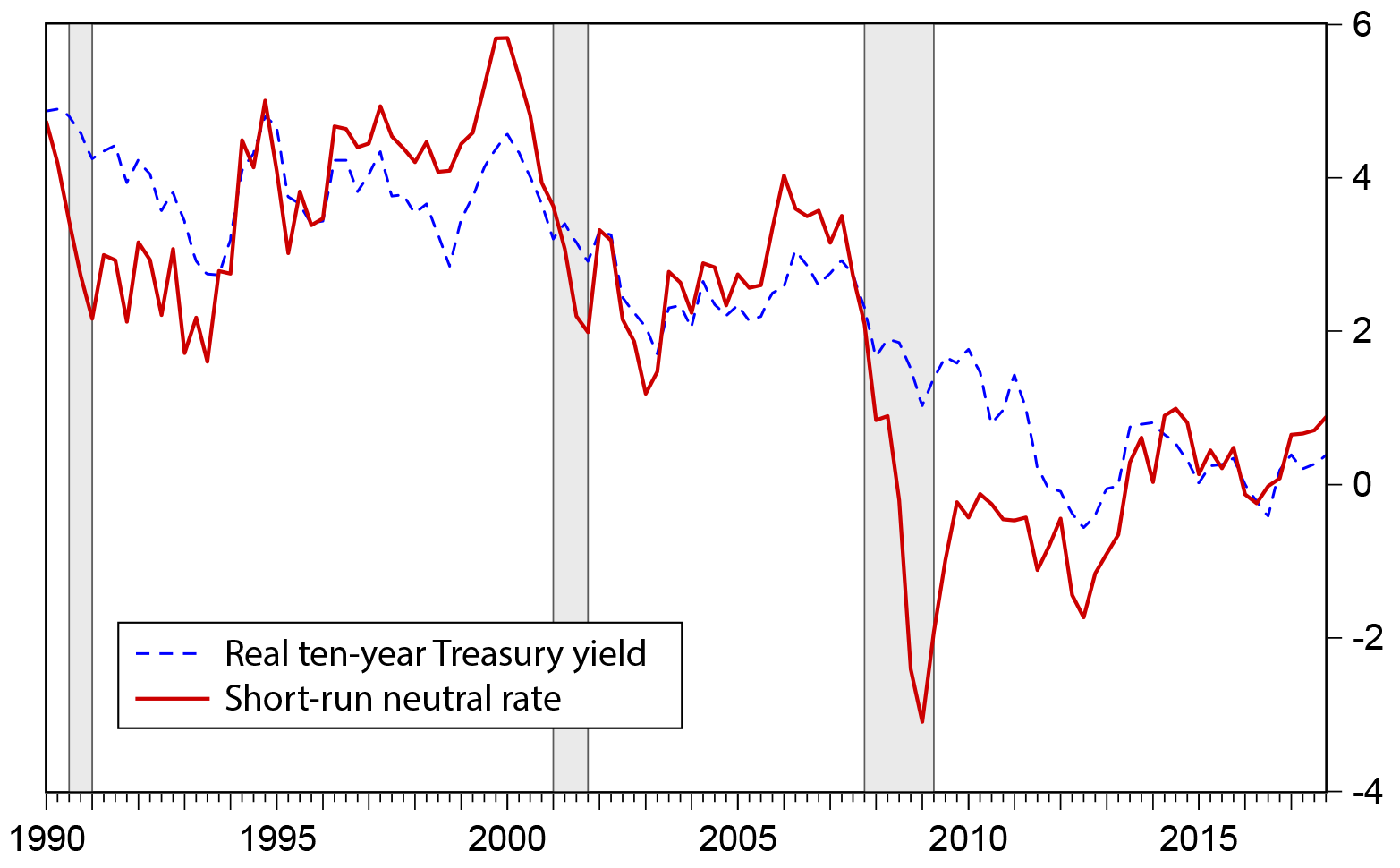
According to this model, the neutral ten-year Treasury yield just prior to the 2008-09 financial crisis was around 3 1/2 percent in real terms. During the crisis, the neutral ten-year Treasury yield dropped as low as 3 percent, in early 2009. By 2010, R_tⁿ had rebounded to around 1/2 percent. Long-term inflation expectations remained stable at around 2 percent during the crisis period, so a real interest rate of 1/2 percent would have been feasible, for example, if the nominal ten-year Treasury yield had dropped to 1 1/2 percent, which could potentially have been achieved through sufficient asset purchases and forward guidance about future short-term interest rates. In 2012, near the peak of the euro crisis, R_tⁿ dipped again, this time to around 1 3/4 percent. Again, such a real ten-year Treasury yield is potentially feasible, because it is lower, in absolute value, than longer-term inflation expectations. By late 2013, R_tⁿ had recovered, and it remained between 1/2 and 1 percent through the end of 2014.

In the couple of years at the end of the sample, the estimate of R_tⁿ has moved up, from around 0 percent in 2016, to just below 1 percent in the last period shown, 2017:Q4. While 1 percent matches the high point since the financial crisis, it is still well below the values that prevailed in the years before the crisis. Of course, the estimates of the neutral rate are only as good as the data underlying them, and this estimate of the output gap, as are all others, is estimated with considerable uncertainty, especially at the end of the sample.

Figure 2 compares the baseline estimate of R_tⁿ with an alternative based on the CBO output gap. The broad contour is similar. In particular, the neutral rate dropped sharply during the crisis and remained depressed relative to pre-crisis levels for many years thereafter. At the end of the sample, there is also a recovery, although using the CBO output gap, R_tⁿ is only about 1/2 percent in 2017:Q4.⁷

Figure 2: The neutral rate of interest with alternative output gaps

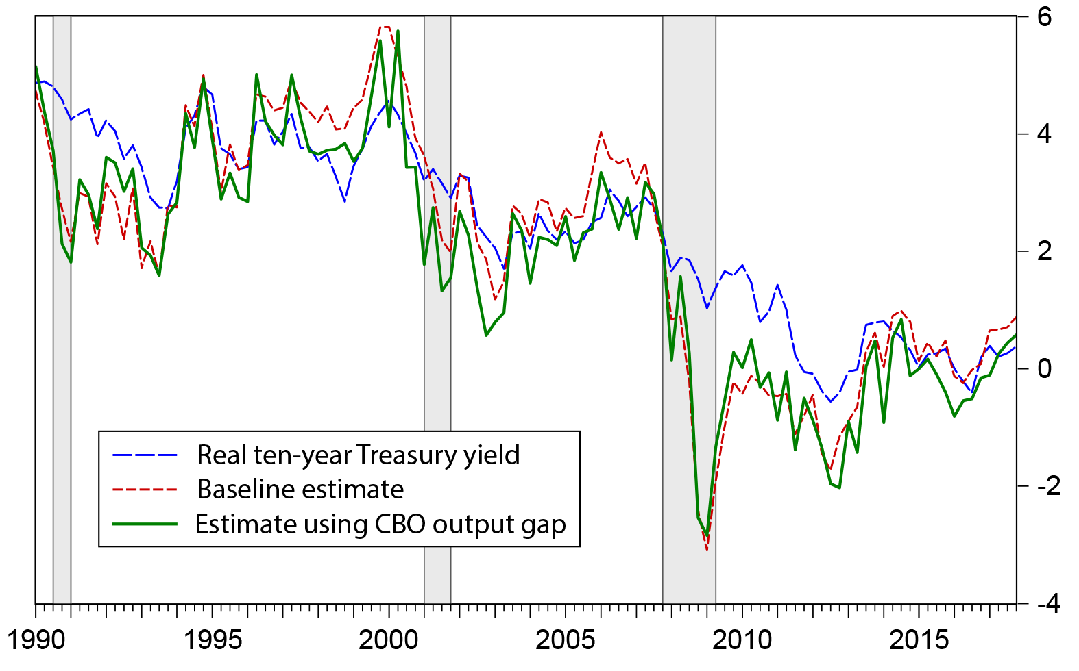
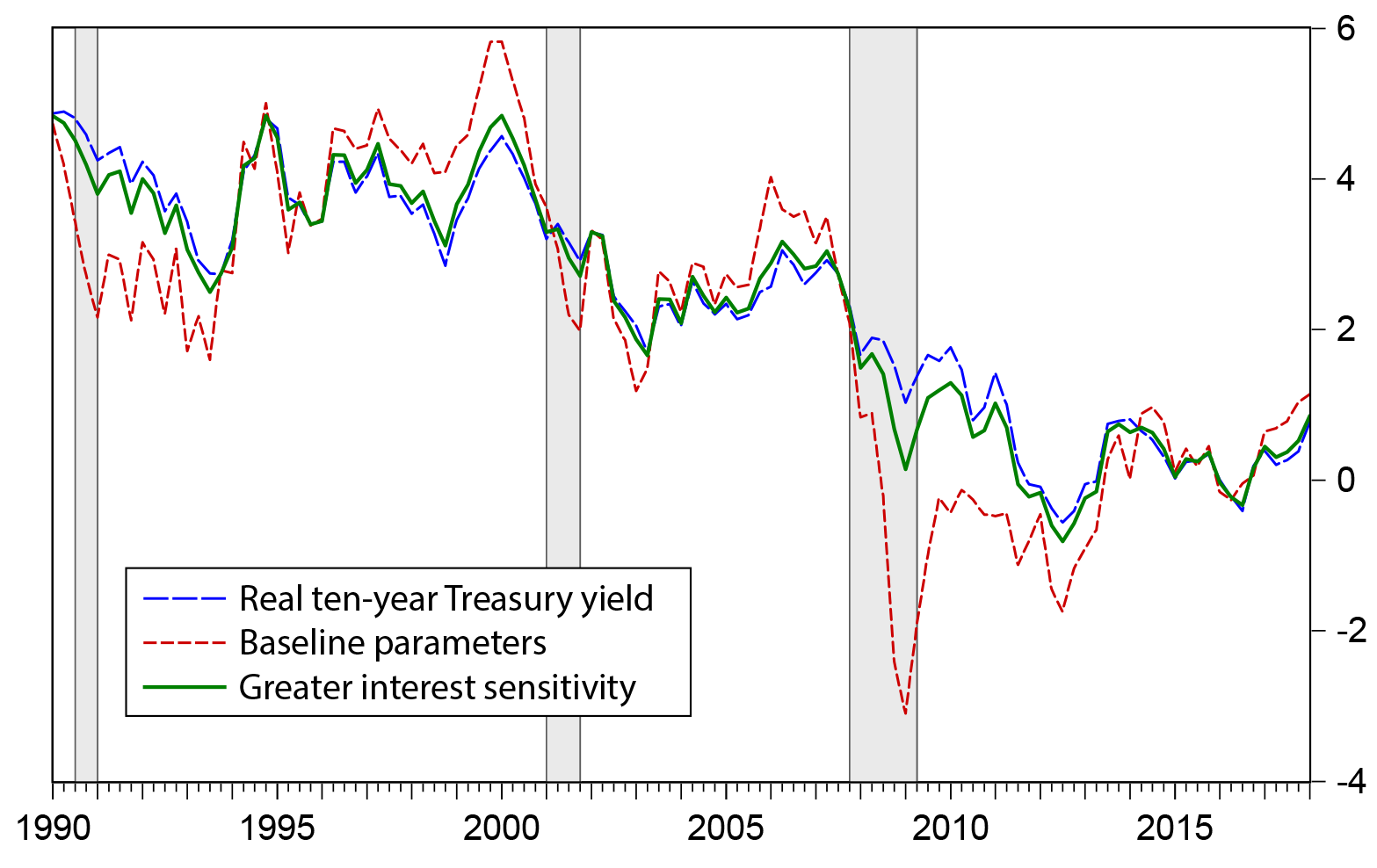
Figure 3 compares the baseline estimate of R_tⁿ, which uses the FRB/US output gap, η = 0.75, and σ = 0.75 with an alternative that assumes η = 0.75, and σ = 3.5. As discussed earlier, with this setting of σ, the interest sensitivity of output is closer to that of DSGE models. Under this alternative, the decline in the real ten-year Treasury yield needed to stabilize the output gap during the financial crisis was considerably smaller than in the baseline case: A real ten-year Treasury yield of about 0 percent would have been sufficient to stabilize the output gap in early 2009, compared with 3 percent under the baseline parameter setting. Under the alternative, the trough of R_tⁿ occurred during the euro crisis, in 2012, when R_tⁿ fell as low as 3/4 percent. Near the end of the sample, both measures show a recovery in R_tⁿ, although the alternative reaches a somewhat smaller value, of around 1/2 percent.

Figure 3: Alternative assumptions about interest sensitivity

There is considerable quarter-to-quarter variation in the estimates of R_tⁿ. One possible source of high-frequency variation is measurement error in the output gap. That possibility is minimized in the preferred estimates, however, because the FRB/US output gap excludes an estimate of measurement error. Another possibility is that the dynamics of the economy are more complex than in equation 1, and this specification error could be reflected in excess high-frequency movements in R_tⁿ.

Figure 4: Smoothing the neutral rate estimate

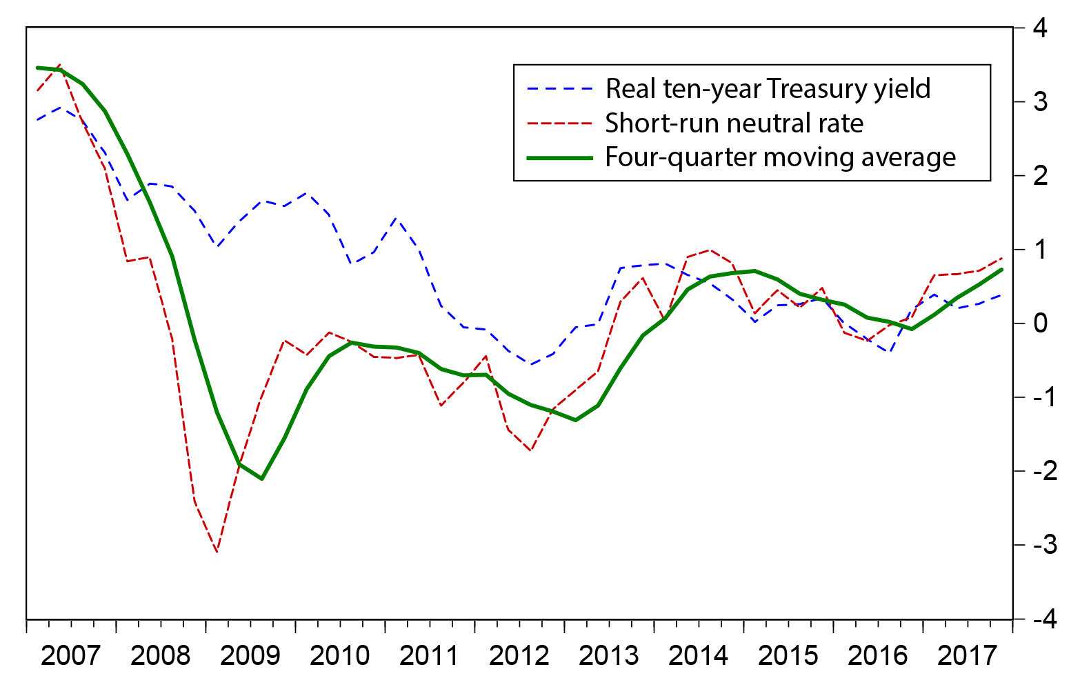
To smooth through high-frequency variation, Figure 4 plots the four-quarter moving average of R_tⁿ. The same broad pattern emerges with, notably, the increase near the end of the sample marking the third period of upward movement since the financial crisis.

The long-run, long-term neutral rate

As has been discussed in a variety of papers, including Kiley (2015), Holston, Laubach, and Williams (2017), and Del Negro et al (2017), the extended period of very low interest rates has raised the prospect that the long-run value of R_tⁿ may have fallen. The estimates of R_tⁿ presented so far have made no assumption about the persistence of the movements in the neutral rate of interest; it is simply the result of applying Equation 2 to the data. Laubach and Williams (2003), and subsequent papers, use the Kalman filter to extract a persistent component of the equilibrium interest rate.

To derive an estimate of the long-run component of the long-term neutral interest rate, we can assume the following state-space model of R_tⁿ:

        R_tⁿ = R_tⁿ + cyc_t ,

        R_tⁿ = R_t-1ⁿ + ε_t ,

       cyc_t = α cyc_t-1 + v_t

As in Laubach and Williams (2003) and other papers in this literature, the long-run component of R_tⁿ, R_tⁿ, follows a random walk. The stationary component, cyc_t, follows an AR(1) process. The residual error terms ε_t and v_t are assumed to follow white noise error processes.

Figure 5: Model estimate of long-run neutral rate

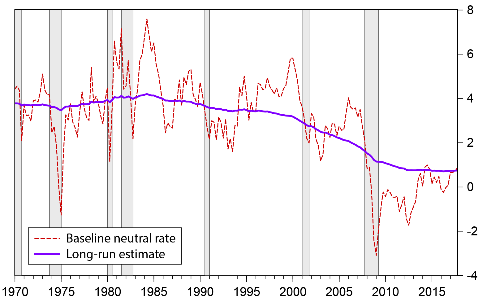
Figure 5 plots the baseline estimate of R_tⁿ along with a model estimate of its long-run component.⁸ In the first twenty years of the sample, the model estimate of the long-run neutral real ten-year Treasury yield fluctuated in a narrow range around 3 3/4 percent. It edged down slightly over the 1990s and more steeply from 1999 to 2011. Over the 2012-to-2017 period, the long-run neutral rate has averaged 3/4 percent, with little variation. This estimate of the long-run neutral interest rate is thus broadly consistent with the results of Holston, Laubach, and Williams (2017), Kiley (2015), and Del Marco et al. (2017), who also find that the long-run neutral interest rate has been lower in recent years than in the decades before the financial crisis.

The gap between the short-run estimate of R_tⁿ and its long-run value, R_tⁿ, can be taken as a measure of the relative aggregate demand facing the economy: When R_tⁿ < R_tⁿ, the level of the real ten-year Treasury yield needed to maintain the output gap at zero is below its long-run value. Such a situation can be characterized as the economy facing "headwinds."⁹ According to the estimates shown in Figure 5, during the financial crisis, in 2008-09, considerable headwinds developed, as R_tⁿ fell well below R_tⁿ. As emphasized by Yellen (2015), these headwinds proved to be persistent, and R_tⁿ remained below R_tⁿ for many years. R_tⁿ briefly exceed R_tⁿ in 2014 but fell back in 2015-16. At the end of the sample, R_tⁿ had once again reached the model estimate of its long-run value. If R_tⁿ were to rise further, so that it exceeded R_tⁿ on a sustained basis, the economy could be said to be benefitting from "tailwinds."¹⁰ Of course, as with any econometric estimate, there is considerable uncertainty around the specific results.

References

Barsky, Robert, Alejandro Justiniano, and Leonardo Melosi (2014). "The Natural Rate of Interest and Its Usefulness for Monetary Policy," American Economic Review 104(5), pp. 37-43.

Board of Governors (2017). FRB/US Model Packages, https://www.federalreserve.gov/econres/us-models-package.htm.

Brainard, Lael (2018). "Navigating Monetary Policy as Headwinds Shift to Tailwinds," speech presented at the Money Marketeers of New York University, New York, New York, March 6, https://www.federalreserve.gov/newsevents/speech/brainard20180306a.htm.

Congressional Budget Office (CBO, 2018). Budget and Economic Outlook: 2018 to 2028, April, https://www.cbo.gov/publication/53651.

Chung, Hess (2015). "The Effects of Forward Guidance in Three Macro Models, FEDS Note 2015-02-26, https://doi.org/10.17016/2380-7172.1488

Curdia, Vasco, Andrea Ferrero, Ging Cee Ng, and Andrea Tambalotti (2015). "Has U.S. Monetary Policy Tracked the Efficient Interest Rate?" Journal of Monetary Economics 70, pp. 72-83.

Del Negro, Marco, Domenico Giannone, Marc P. Giannoni, and Andrea Tambalotti (2017). "Safety, liquidity, and the natural rate of interest," Brookings Papers on Economic Activity, Spring 2017, pp. 235-294, https://www.brookings.edu/wp-content/uploads/2017/08/delnegrotextsp17bpea.pdf.

Edge, Rochelle M., Michael T. Kiley, and Jean-Philippe Laforte (2008). "Natural Rate Measures in an Estimated DSGE Model of the U.S. Economy," Journal of Economic Dynamics and Control 32, pp. 2512-2535.

Fleischman, Charles, and John M. Roberts (2011). "From Many Series, One Cycle: Improved Estimates of the Business Cycle from a Multivariate Unobserved Components Model, Finance and Economics Discussion Series 2011-46, Board of Governors of the Federal Reserve System, https://www.federalreserve.gov/pubs/feds/2011/201146/201146abs.html.

Holston, Kathryn, Thomas Laubach, and John C. Williams (2017). "Measuring the Natural Rate of Interest: International Trends and Determinants," Journal of International Economics 108, May 2017, S59-S75, https://www.frbsf.org/economic-research/publications/working-papers/2016/wp2016-11.pdf

Kiley, Michael T. (2015). "What Can the Data Tell Us About the Equilibrium Real Interest Rate?" Finance and Economics Discussion Series 2015-077. Board of Governors of the Federal Reserve System (U.S.).

Laubach, Thomas, and John C. Williams (2003). "Measuring the Natural Rate of Interest," Review of Economics and Statistics, 85(4), November, pp. 1063-1070.

Powell, Jay (2018). "Statement on the Semiannual Monetary Policy Report to the Congress," testimony before the Committee on Financial Services, U.S. House of Representatives, Washington, D.C., February 27, https://www.federalreserve.gov/newsevents/testimony/powell20180226a.htm.

Roberts, John M. (2014). "Estimates of Latent Variables for the FRB/US Model," available at the Federal Reserve Board's Public FRB/US website, https://www.federalreserve.gov/econres/us-models-package.htm.

Smets, Frank, and Rafael Wouters (2007). "Shocks and Frictions in U.S. Business Cycles: A Bayesian DSGE Approach," American Economic Review 97, pp. 586-606, https://www.aeaweb.org/articles?id=10.1257/aer.97.3.586.

Woodford, Michael (2003). Interest and Prices, Princeton University Press.

Yellen, Janet (2015). "Normalizing Monetary Policy: Prospects and Perspectives," speech presented at "The New Normal Monetary Policy," a research conference sponsored by the Federal Reserve Bank of San Francisco, San Francisco, California, March 27, https://www.federalreserve.gov/newsevents/speech/yellen20150327a.htm.