FEDS Notes
December 21, 2018
Factors in Unemployment Dynamics1
Hie Joo Ahn and James Hamilton (University of California, San Diego)
The U.S. unemployment rate averaged 8.4% during the first five years of recovery from the Great Recession of 2007-2009, the weakest recovery on record (see Figure 1). But as the expansion continued, unemployment continued to decline and by 2018 reached the lowest levels in almost half a century. Why did unemployment remain so high for so long, and what factors contributed to the recent lows?
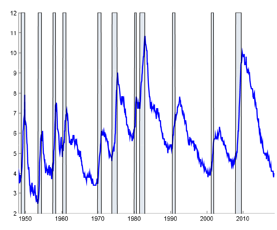
Source: U.S. Bureau of Labor Statistics.
One of the most striking features of the length of time people stay unemployed is the heterogeneity across the experience of different people. Most people who become unemployed find a new job relatively quickly. Even during the Great Recession, of people who were newly unemployed in month t, on average only 64% were still unemployed in month t + 1. By contrast, if someone has been unemployed for 4-6 months as of month t, on average since 1976, there was an 81% probability that they would still be unemployed in month t + 1. The lowest the latter probability ever got in any month from 1976 to 2018 was 71%. In other words, the newly unemployed during the Great Recession had better success finding jobs than did the long-term unemployed during the strongest economic boom.
Why do the long-term unemployed have such a dramatically lower probability of exiting unemployment? One possibility is that the experience of being unemployed directly changes the individual. Loss of job experience or discrimination by potential employers could lead to a lower likelihood of being hired. A field experiment by Kroft, Lange and Notowidigdo (2013) found some evidence of discrimination against the long-term unemployed. However, an audit study by Farber, Silverman, and von Wachter (2015) found no relation between unemployment duration and employer call-back rates, and Jarosch and Pilossoph (2018) demonstrated that findings of discrimination like those of Kroft, Lange and Notowidigdo (2013) could readily be explained by true ability differences across individuals that are signaled by longer spells of unemployment.
Another factor accounting for the differences in the unemployment-continuation probabilities between the newly unemployed and the long-term unemployed is unobserved heterogeneity. Suppose some individuals start out with a high probability of exiting unemployment and others with a lower probability. As we look at a pool of individuals who have been looking for work for n months, the latter individuals will make up a larger fraction of the pool as n increases, accounting for the observed tendency of the unemployment-continuation probability to increase with n. Suppose for example that 80% of the newly unemployed (whom we will call type H) have a continuation probability of 35% and the remaining 20% (type L) have a continuation probability of 85%. Figure 2 tracks the number of individuals Un who are still unemployed at each duration n along with the average unemployment-continuation probability predicted for each group. As n increases, type L make up a larger share of the remaining group of unemployed, causing the average unemployment-continuation probability to rise with n.
Figure 2: Ex ante heterogeneity can cause observed unemployment-continuation probabilities to increase with duration
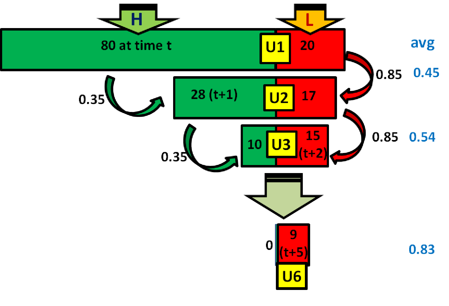
Source: Ahn and Hamilton (forthcoming).
The numbers in Figure 2 were calibrated to match the average continuation probabilities observed for each group n since 1976. We could alternatively choose to match the average numbers observed during and right after the Great Recession (2007:12 to 2013:12). When we do this, we impute a slight increase in the continuation probability of type L individuals (from 85% to 89%) and a big increase in the fraction of type L among the newly unemployed (from 20% to 32%), as seen in Figure 3.
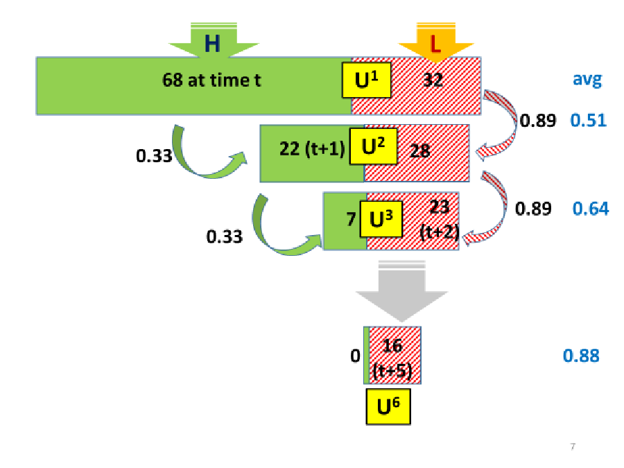
Source: Numbers represent new inflows and unemployment-continuation probabilities calibrated to average counts of unemployed by duration over 2007:12 through 2013:12. Calculated using parameters in row 7 of Ahn and Hamilton (forthcoming).
Ahn and Hamilton (forthcoming) showed how a similar calibration exercise can be updated on a month-to-month basis using a formal statistical model. We allowed both the number of new inflows of type L and type H (which we denote wLt and wHt) as well as the unemployment-continuation probabilities for a newly unemployed individual for each type (pLt(1) and pHt(1)) to change every month t according to a random walk. We also allowed for the possibility of a direct effect of duration itself on continuation probabilities using a proportional hazards specification, in which the continuation probability for a type L individual who has been unemployed for n months as of date t (pLt(n)) is a product of two functions, the first of which (pLt(1)) depends on the date t but not the duration of unemployment n, and the second depends on n but not t. The dependence on n was completely general--rising duration could increase the unemployment-continuation probability over some ranges and decrease it over others. However, we assumed that whatever the form of this function, it is constant over time and interacts with the unobserved heterogeneity according to the proportional-hazards specification. This framework turns out to imply a nonlinear state-space model with which the likelihood function of observed counts of unemployed by each duration n can be calculated and an optimal inference about wLt, wHt, pLt(n), and pHt(n) for each month t obtained.
Our estimates suggest that the direct effects on unemployment-continuation probabilities of the length of time people have been unemployed are relatively modest. We attribute most of the observed correlation between duration and continuation probability to the effect of dynamic sorting illustrated in Figure 2.
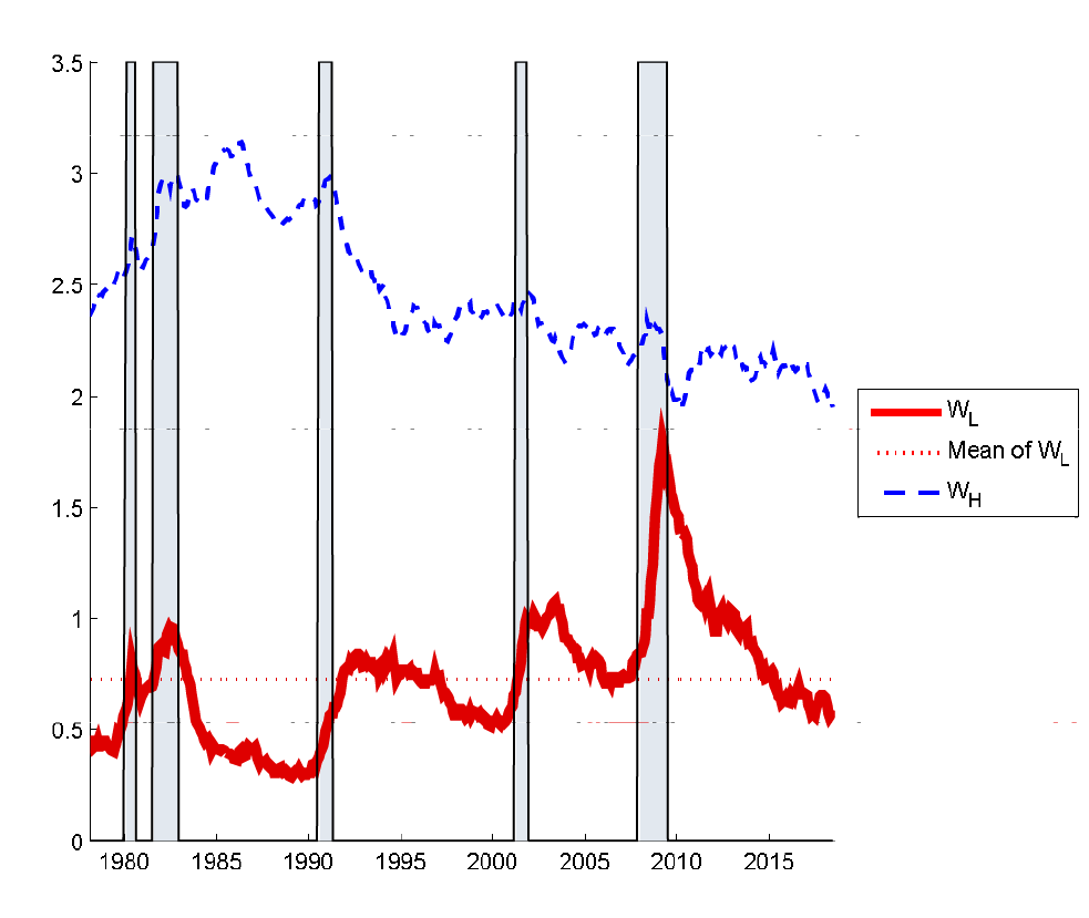
Our estimates of the unemployment-continuation probabilities for newly unemployed workers of each type (pLt(1) and pHt(1)) are plotted in Figure 4. These average 0.82 and 0.35, respectively, consistent with the calibration to the full sample numbers in Figure 2. We find a tendency of pLt(1) to increase during recessions and a modest decline in pHt(1) since 1990--recently type H individuals have if anything spent even less time unemployed than was the case historically.
Figure 4: Unemployment-continuation probabilities for newly unemployed individuals of each type, 1978:1-2018:6
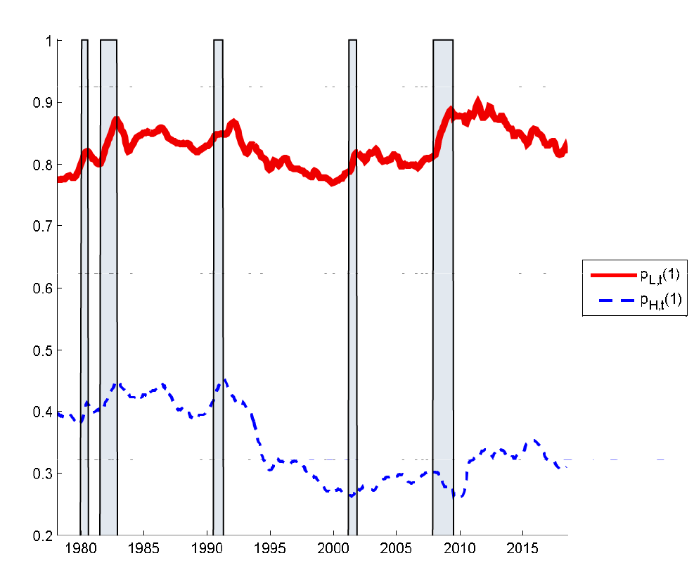
Source: Updated by the authors following procedure in Ahn and Hamilton (forthcoming).
Figure 5 plots our estimates for the monthly inflows into unemployment of each type (wLt and wHt). We find a downward trend in the inflows of type H individuals, consistent with the conclusion that the labor market has become less dynamic over time with less "churning" of workers between jobs (Bleakley, Ferris and Fuhrer, 1999). The key factor that seems to change in recessions is a big increase in the inflow into unemployment of type L individuals.
Figure 5: Monthly number of newly unemployed individuals of each type (million workers), 1978:1-2018:6
Source: Updated by the authors following procedure in Ahn and Hamilton (forthcoming).
Why did unemployment remain so high during the first five years of the recovery from the Great Recession? Figure 5 provides a clear answer: new inflows into unemployment of type L individuals remained well above their historical average levels until 2014. Given that these individuals tend to stay unemployed for so long, this kept unemployment well above historical average levels. Since 2014, type L inflows have been significantly below average, and this is what has finally brought unemployment down.
Another feature of our model is that it allows us to do a historical decomposition of the various factors contributing to changes in the unemployment rate. Given our inference about the values of all the variables in 2014:1, the dynamic model generates a multi-step-ahead forecast of the unemployment rate for every month since then. This forecast (a modest ongoing decline in the unemployment rate) is shown as the thin black line in Figure 6. The actual drop in unemployment (the thicker black RU line) turned out to proceed much more rapidly and eventually reach much lower levels than the model would have predicted in 2014:1. Our model can attribute this ex post forecast error to unanticipated changes in the four driving variables wLt, wHt, pLt(1), and pHt(1). The contributions of these four shocks are shown as the red starred, solid fuchsia, blue circled, and dotted green lines, respectively. The distance between each line and the thin black line shows the contribution to the change in the variable relative to 2014:1.2 By far the most important factor bringing the unemployment rate down has been fewer new inflows of type L individuals. Slightly lower unemployment-continuation probabilities for those individuals also made a modest contribution.
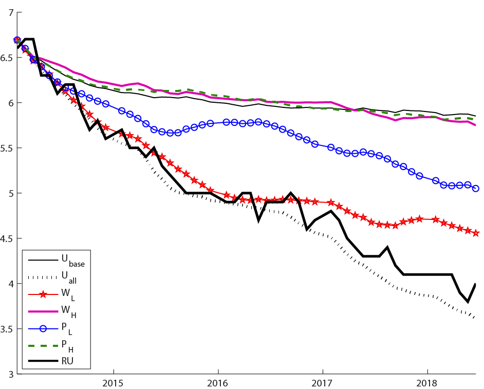
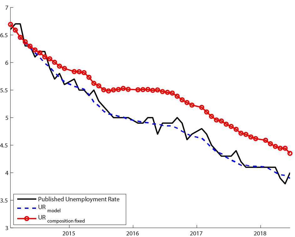
Figure 7 reports an alternative counterfactual calculation. The solid black line is the actual unemployment rate and the dashed blue line is the fitted rate from our model; deviations between these two are interpreted by our framework as measurement error in the data. The dashed red line is a counterfactual for what the unemployment rate would have been if the total inflows into unemployment and outflow rates for each month were the same as observed in the data but the fraction of type L inflows into unemployment remained fixed at its 2014:1 value. The unemployment rate today would be 0.5% higher under this counterfactual scenario.
And who are the type L workers? Ahn (2018) used this framework to examine the role of a variety of observed characteristics of the unemployed, including gender, age, education, industry, and reason for unemployment. No matter what observable characteristics one conditions on, the dramatic differences in unemployment-continuation probabilities between the newly unemployed and the long-term unemployed are still found, indicating that there are significant numbers of those we would designate type L among any demographic group of newly unemployed individuals. The one observable characteristic that seems most closely related to the type L designation is the reason people gave for why they were unemployed. The key category is involuntary permanent separations--people who lost their job with no indication of a recall and are now looking for another job. These individuals are known to have a much harder time finding a new job than those who become unemployed for other reasons (Bednarzik, 1983; Fujita and Moscarini, 2017). Since 1994, the unemployment-continuation probability for individuals who were newly unemployed as a result of involuntary permanent separation was 76%, much higher than the average for other newly unemployed individuals. Ahn (2018) concluded that permanent job losers who are type L account for around 50% of the aggregate type L unemployment and drive most of its cyclicality. Figure 8 plots the monthly number of new involuntary permanent separations. Like our series for WLt, these remained elevated for many years after the recovery from the Great Recession began.
Figure 8: Newly unemployed individuals who listed involuntary permanent separation as the reason (thousand workers), 1994:1 to 2018:6
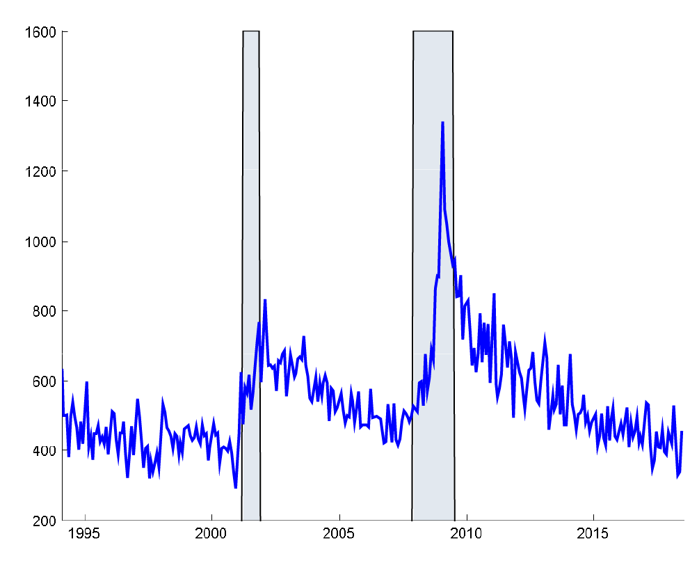
Source: U.S. Bureau of Labor Statistics.
What are the implications for policy? When product demand falls, firms may first choose to shed the least productive workers and those whose skills are not currently in demand. Expansionary fiscal or monetary policy that boosts aggregate demand might help those individuals return to work. On the other hand, strong labor demand or an expansionary policy cannot really change an individual's characteristics, and do not reverse skill-biased technological change. Thus, employment recoveries will be slower, for a given amount of labor demand, if the share of type L unemployment is higher. As a result, increases in the share of type L unemployment can be thought of as adverse shocks to the functioning of the labor market.
Ahn (2018) found some evidence that is consistent with the second interpretation. She started with a Phillips Curve specification similar to that in Coibion and Gorodnichenko (2015) in which the gap between inflation $$\pi_t$$ and the level of inflation expected from the Michigan survey $$\pi^*_t$$ in quarter t is explained by the gap between the unemployment rate ut and the CBO estimate of the natural rate of unemployment $$u_t^*$$ along with lags of the inflation gap. She then added the number of unemployed type L workers UtL as a fraction of the labor force Nt as an additional explanatory variable to the Phillips Curve (standard errors in parentheses): $$$$ \pi_t-\pi_t^* = c + \sum_{j=1}^8 \beta_j (\pi_{t-j}-\pi_{t-j}^*) - \underset{(0.139)}{0.445}\ (u_t-u_t^*) + \underset{(0.117))}{0.273}\ \frac{U_t^L}{N_t} +e_t $$$$ for t = 1980:Q1 to 2018:Q2. Notice that $$\frac{U_t^L}{N_t}$$ enters with the same sign but slightly smaller magnitude as the natural rate of unemployment suggesting that permanently separated type L unemployment has information that can be useful for predicting inflation beyond that contained in the conventional measure of the natural rate of unemployment. The ratio $$\frac{U_t^L}{N_t}$$ declined from 4.6% in 2014:1 to 2.2% today, which would lead the above equation to predict 0.273(4.6-2.2)=0.65% lower inflation than expected on the basis of the observed declines in the total unemployment rate ut and natural unemployment rate $$u_t^*$$ alone. Another way to summarize this finding is that the natural rate of unemployment $$u_t^*$$ may have declined even more than the 0.4% drop since 2014:1 estimated by the Congressional Budget Office.
References
Ahn, Hie Joo (2018). "The Role of Observed and Unobserved Heterogeneity in the Duration of Unemployment Spells," Working paper.
Ahn, Hie Joo, and James D. Hamilton (forthcoming). "Heterogeneity and Unemployment Dynamics," Journal of Business and Economic Statistics.
Bednarzik, Robert (1983). "Layoffs and Permanent Job Losses: Workers' Traits and Cyclical Patterns," Monthly Labor Review, September: 3-12.
Bleakley, Hoyt, Ann E. Ferris, and Jeffrey C. Fuhrer (1999). "New Data on Worker Flows During Business Cycle," New England Economic Review, July/August: 49-76.
Coibion, Olivier, and Yuriy Gorodnichenko (2015). "Is the Phillips Curve Alive and Well After All? Inflation Expectations and the Missing Disinflation," American Economic Journal: Macroeconomics 7: 197-232.
Farber, Henry S., Dan Silverman, and Till von Wachter (2015). "Factors Determining Callbacks to Job Applications by the Unemployed: An Audit Study," NBER working paper 21689.
Fujita, Shigeru, and Giuseppe Moscarini (2017). "Recall and Unemployment," American Economic Review 107, no. 12: 3875-3916.
Jarosch, Gregor, and Laura Pilossoph (2018). "Statistical Discrimination and Duration Dependence in the Job Finding Rate," NBER working paper 24200.
Kroft, Kory, Fabian Lange, and Matthew J. Notowidigdo (2013). "Duration Dependence and Labor Market Conditions: Evidence from a Field Experiment," Quarterly Journal of Economics 128, no. 3: 1123-1167.
1. We thank Travis Berge, Andrew Figura, Charles Fleischman, and Glenn Follette for helpful comments. The views expressed in this note are those of the authors only and do not necessarily represent those of the Federal Reserve Board or its staff. Return to text
2. The sum of these four lines (shown as the dotted black line) does not equal the actual unemployment rate because our framework also allows for measurement errors in the measured counts of unemployed individuals by each duration. There is also a linearization error that grows with the length of the horizon being forecast. Return to text
3. The specification differs slightly from that in Coibion and Gorodnichenko in that Ahn's specification also adds lags of inflation. Return to text
Ahn, Hie Joo, and James Hamilton (2018). "Factors in Unemployment Dynamics," FEDS Notes. Washington: Board of Governors of the Federal Reserve System, December 21, 2018, https://doi.org/10.17016/2380-7172.2274.
Disclaimer: FEDS Notes are articles in which Board staff offer their own views and present analysis on a range of topics in economics and finance. These articles are shorter and less technically oriented than FEDS Working Papers and IFDP papers.