FEDS Notes
May 24, 2019
Weekly Hours, Overtime, and Employment of Manufacturing Production Workers: Fluctuations over the Business Cycle
Employment, weekly hours, and overtime hours are all highly cyclical indicators of economic activity. Of these three measures of labor inputs, changes in employment, however, tend not to be a firm’s first response to changes in demand due to the costs of labor adjustment. As a result, firms typically adjust their employees’ hours of work before changing employment. This response has been so cyclically consistent that average weekly hours of production workers has appeared on the list of leading indicators since it was first developed by Mitchell and Burns (1938).
This note analyzes how weekly hours, overtime, and employment of production workers move over the business cycle. We restrict our focus to the manufacturing sector because, despite representing only about 11 percent of the U.S. economy, it is among the most sensitive industries to business cycle fluctuations. Our analysis relies on monthly data on employment, average weekly hours, and overtime hours of manufacturing production workers published by the Bureau of Labor Statistics (BLS). Because of data availability, our sample starts in 1956 and covers eight recessions.2
Figure 1 presents the average movements of weekly hours, overtime, and employment over a 24-month window around business cycle turning points. For ease of comparison, all series are scaled by their average level during peaks; in addition, we normalize their values at NBER peaks (left panel) and troughs (right panel) to identify percentage changes relative to the turning point.
Figure 1a: Response of Employment, Weekly Hours, and Overtime of Manufacturing Production Workers around Recessions
Business Cycle Movements around Trough
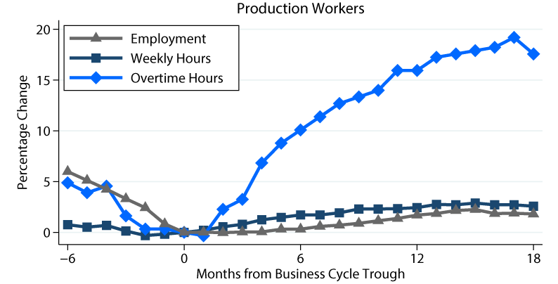
Figure 1b: Response of Employment, Weekly Hours, and Overtime of Manufacturing Production Workers around Recessions
Business Cycle Movements around Peak
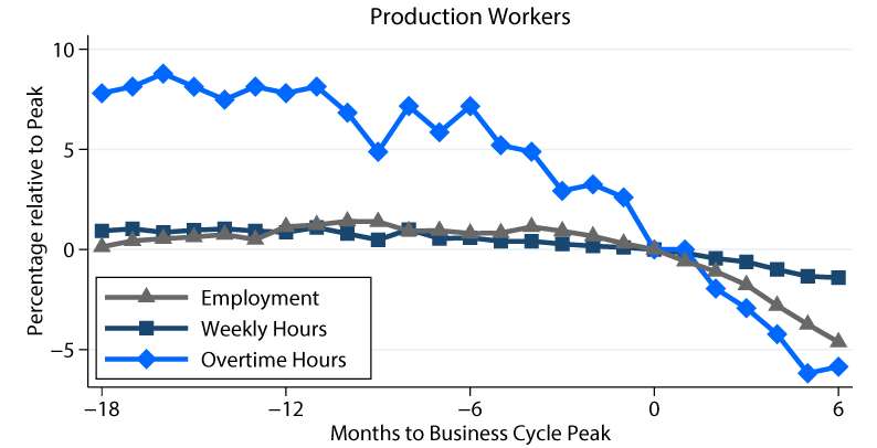
Note: Percentage change in average weekly hours, average overtime hours, and employment of production workers relative to average peak, 1956 to 2018. NBER business cycles troughs are normalized to zero.
Source: Bureau of Labor Statistics (BLS)
Overtime hours appear most responsive to business cycle fluctuations: Six months before the business cycle peak, overtime hours are 7 percent above their value at the business cycle peak and start to decline significantly (figure 1a); similarly, six months after the business cycle trough, overtime hours recover swiftly with a 10 percent increase (figure 1b). Both weekly hours and employment, instead, tend to move more modestly around turning points, wavering around a few percentage points, but each follows different timing: Fluctuations in weekly hours closely mirror the timing of changes in overtime, while the response of employment appears somewhat delayed, especially during a recovery. This finding is consistent with the presence of adjustment costs related to hiring and firing workers, which induce firms to respond cautiously to changes in demand by adjusting overtime and straight-time hours first.
Figure 2 confirms the cyclical properties of overtime hours. We isolate the cyclical components of weekly hours, overtime, and employment using a Baxter-King filter. Overtime hours display the largest swings around recessions; additional fluctuations, however, are present during expansions, likely unrelated to aggregate business cycle movements.
Figure 2: Cyclical Variation of Employment, Weekly Hours, and Overtime of Manufacturing Production Workers
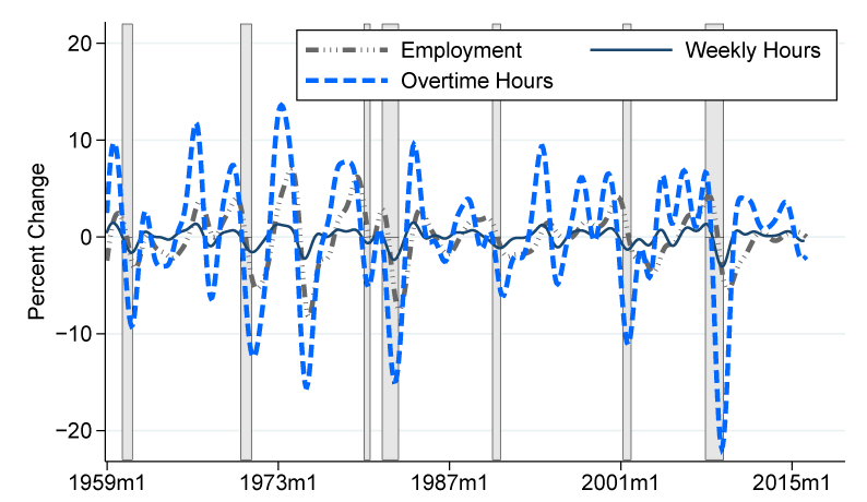
Note: Cyclical components from Baxter-King filter; each series is normalized by its average peak. Gray-shaded areas indicate NBER recession periods: April 1960–February 1961, December 1969–November 1970, January 1980–July 1980, July 1981–November 1982, July 1990–March 1991, March 2001–November 2001, December 2007–June 2009.
Source: BLS.
To identify more precisely the business cycle properties of weekly hours, overtime, and employment, we look at their correlation with an indicator of the business cycle. Rather than targeting a single business cycle proxy, we have constructed an aggregate indicator based on five underlying series—real GDP, real personal income less transfers, real manufacturing and wholesale–retail trade sales, manufacturing production, and nonfarm employment—used by the NBER Business Cycle Dating Committee to identify the December 2007 peak.3, 4 Figure 3 shows the correlation function for weekly hours, overtime, and changes in employment at different business cycle leads. We calculate the correlation at a quarterly frequency to smooth through the monthly volatility. All series display the highest correlation at zero leads—i.e., with the contemporaneous change in our business cycle indicator—suggesting a high sensitivity to coincident business cycle movements. In particular, the correlation between our business cycle indicator and overtime hours is around 0.76 at zero leads. An even slightly higher correlation applies to changes in employment: While labor market adjustments through layoffs and hiring tend to occur at a slower pace than changes to overtime before peaks and after troughs, they tend to catch up over time as the economic activity continues to contract or expand. The correlation coefficients decline at higher leads of the labor market series, following a similar trend across all three series, and are not significantly different from zero for the six-quarter-ahead variables (at six leads).
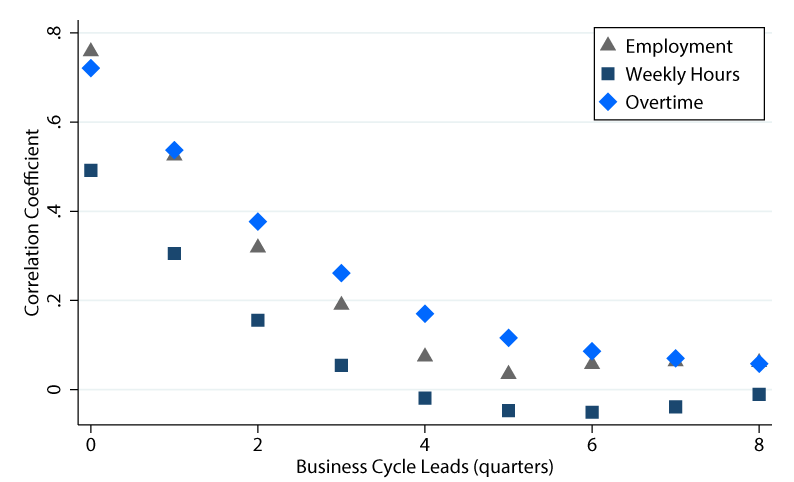
Note: Correlation between an index of the business cycle and leads of employment, weekly hours, and overtime hours.
Source: BLS, Census, FRB, MacroAdvisors, and Stock & Watson.
Cyclical movements, however, are not synchronous across all manufacturing industries. Table 1 highlights the sector-level differences in the pattern of contemporaneous correlations with our business cycle indicator; the table displays the correlation between changes in employment, weekly hours, and overtime for each three-digit NAICS sector with available data. The pattern of correlation differs not only across industries but also across labor market series. Looking at the average correlation across the three indicators, Transportation Equipment and Wood Manufacturing are the most sensitive sectors to business cycle movements, while Petroleum and Coal Products and Food Manufacturing seem the least responsive to changes in economic activity.
Table 1: Sector Correlations
| Correlations | |||||
|---|---|---|---|---|---|
| NAICS | Sector | Employment | Weekly Hours | Overtime | Average |
| 311 | Food | 0.23 | -0.05 | 0.27 | 0.15 |
| 313 | Textile Mills | 0.37 | 0.61 | 0.64 | 0.54 |
| 314 | Textile Prod | 0.52 | 0.40 | 0.60 | 0.51 |
| 315 | Apparel | 0.02 | -0.08 | 0.53 | 0.16 |
| 321 | Wood | 0.78 | 0.58 | 0.49 | 0.62 |
| 322 | Paper | 0.57 | 0.49 | 0.59 | 0.55 |
| 323 | Printing | 0.63 | 0.42 | 0.49 | 0.51 |
| 324 | Petroleum & Coal | 0.29 | -0.11 | 0.08 | 0.09 |
| 325 | Chemicals | 0.43 | 0.61 | 0.56 | 0.53 |
| 326 | Plastics | 0.76 | 0.33 | 0.68 | 0.59 |
| 327 | Nonmetallic Prod | 0.71 | 0.27 | 0.55 | 0.51 |
| 331 | Primary Metals | 0.69 | 0.60 | 0.52 | 0.61 |
| 332 | Fabricated Metal | 0.74 | 0.50 | 0.59 | 0.61 |
| 333 | Machinery | 0.62 | 0.50 | 0.66 | 0.59 |
| 334 | Electronics | 0.48 | 0.42 | 0.50 | 0.47 |
| 335 | Electrical Eq | 0.51 | 0.50 | 0.41 | 0.47 |
| 336 | Transportation Eq | 0.72 | 0.63 | 0.73 | 0.70 |
| 337 | Furniture | 0.81 | 0.39 | 0.56 | 0.59 |
| 339 | Miscellaneous | 0.57 | 0.24 | 0.56 | 0.46 |
Note: Contemporaneous correlations between business cycle aggregate indicator and the labor market conditions series (employment, weekly hours, overtime).
To isolate the signal of more cyclical industries, we leverage on the three-digit sector-level correlation properties to construct an estimate of movements in our business cycle indicator. With potentially large numbers of predictors—including all three-digit sector-level data on employment, weekly hours, and overtime as well as possible various lags—we rely on Lasso-based techniques to address the model selection problem.5 Following Belloni and Chernozhukov (2013), we then use the OLS post-Lasso estimator to construct our prediction of the business cycle indicator. Finally, we evaluate its performance around recessions not included in the sample used for estimation.6
1980s Recessions
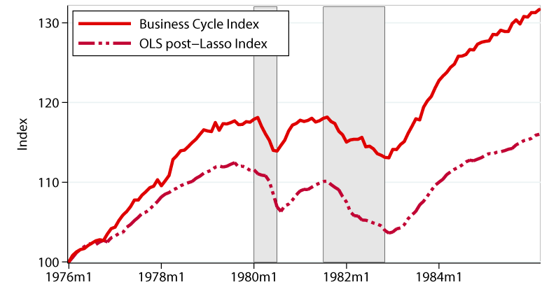
Note: Comparison between a business cycle indicator and an OLS post-Lasso-based index of weekly hours, overtime, and employment in selected industries. Indicators are normalized to 100 in 1976m1.
Source: BLS, Census, FRB, MacroAdvisors, and Stock & Watson.
1990 Recession
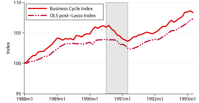
Note: Comparison between a business cycle indicator and an OLS post-Lasso-based index of weekly hours, overtime, and employment in selected industries. Indicators are normalized to 100 in 1988m1.
Source: BLS, Census, FRB, MacroAdvisors, and Stock & Watson.
Figure 4 compares our business cycle indicator with the out-of-sample prediction implied by our methodology. While the trends of the two series are remarkably different in the 1980s, we mostly focus on the ability of our prediction to identify business cycle turning points. In particular, our prediction points to declines in economic activity that coincide with the onset of recessions in two out of the three cases shown in figure 4. While in the 1980s our estimate seems well synchronized with the fluctuations in the business cycle indicator around recessions (figure 4a), in the 1990s our indicator remains flat for a few months before declining well after the March 1991 recession begins.
Overall, employment, weekly hours, and overtime of manufacturing production workers provide some signal on business cycle fluctuations, but a prediction that builds on detailed sector-level data is far from accurate. The mediocre performance could partly be attributed to the fact that the dating committee characterizes recessions as "a broad contraction of the economy, not confined to one sector" and, thus, "emphasizes economy-wide measures of economic activity." A second caveat applies to the evaluation of our prediction: Our analysis relies on fully revised data; with the unfeasibility of collecting all vintages of past data revisions, how would the business cycle properties of the labor market series and predictions change with real-time data remains the topic of ongoing evaluation.
References
Belloni, Alexandre, and Victor Chernozhukov (2013). "Least Squares after Model Selection in High-Dimensional Sparse Models," Bernoulli, 19 (2), pp. 521–47.
Business Cycle Dating Committee, National Bureau of Economic Research (2008). "Determination of the December 2007 Peak in Economic Activity," December 1 (revised December 11, 2008), https://www.nber.org/cycles/dec2008.html.
Federal Reserve Bank of St. Louis (2019). FRED Economic Data, BEA series W875RX1, St. Louis Fed series CMRMTSPL, BLS series PAYEMS, https://fred.stlouisfed.org/tags/series (accessed May 3, 2019).
Board of Governors of the Federal Reserve System (2019). Statistical Release G.17, "Industrial Production and Capacity Utilization" (April 16), https://www.federalreserve.gov/releases/g17/Current/.
Macroeconomic Advisers (2018). "U.S. Monthly GDP Index," https://ihsmarkit.com/products/us-monthly-gdp-index.html (accessed May 3, 2019).
Mitchell, Wesley C., and Arthur F. Burns (1938). "Statistical Indicators of Cyclical Revivals," NBER Bulletin, no. 69 (New York: National Bureau of Economic Research, May 28). Reprinted in Geoffrey H. Moore, ed. (1961). Business Cycle Indicators, vol. 1: Contributions to the Analysis of Current Business Conditions. Princeton, N.J.: Princeton University Press, pp. 163–83.
Stock, James H., and Mark W. Watson (2010). "Distribution of Quarterly Values of GDP/GDI across Months within the Quarter," memorandum, Princeton University, September 19, http://www.princeton.edu/~mwatson/mgdp_gdi/Monthly_GDP_GDI_Sept20.pdf.
1. The views expressed in the article are those of the author and do not necessarily reflect those of the Federal Reserve System. I would like to thank Vivi Gregorich for excellent research assistance. Kim Bayard, Leland Crane, and Charlie Gilbert provided extensive resources and guidance for this project. Return to text
2. Following the National Bureau of Economic Research (NBER)'s recession dating, our sample includes the following recessions: August 1957–April 1958, April 1960–February 1961, December 1969–November 1970, January 1980–July 1980, July 1981–November 1982, July 1990–March 1991, March 2001–November 2001, December 2007–June 2009. Return to text
3. In its memorandum on the December 2007 peak, the NBER's Dating Committee indicated that it considers real GDP, real personal income less transfers, real manufacturing and wholesale–retail trade sales, industrial production, and nonfarm employment to date business cycle turning points. We replaced industrial production with manufacturing production primarily because the volatility in total IP reflects weather factors and fluctuations in the mining sector, which tend not to be well aligned with economy-wide business cycle fluctuations. Return to text
4. To maintain monthly indicators, we construct a monthly GDP series that relies on the estimates developed by Stock and Watson (2010) and by Macroeconomic Advisors (2018). Other monthly indicators have been accessed via the FRED database (real personal income excluding current transfer receipts [W875RX1], real manufacturing and trade industries sales [CMRMTSPL], all employees: total nonfarm payrolls [PAYEMS]). Return to text
5. Specifically, we use a three-step-ahead cross-validation Lasso method to select our model. This methodology selects 15 regressors: average weekly hours for textile products, for petroleum and coal products, and for chemicals; changes in employment for wood products (one- and two-month lags), for cement and glass products, for primary metals, for fabricated metals, for transportation equipment, for furniture, and for miscellaneous products (two-month lag); and overtime hours for textile products, for cement and glass products, and for transportation equipment. Return to text
6. We implement our model selection methodology on a restricted sample, 1992m1 to 2018m12. Return to text
Tito, Maria D. (2019). "Weekly Hours, Overtime, and Employment of Manufacturing Production Workers: Fluctuations over the Business Cycle," FEDS Notes. Washington: Board of Governors of the Federal Reserve System, May 24, 2019, https://doi.org/10.17016/2380-7172.2385.
Disclaimer: FEDS Notes are articles in which Board staff offer their own views and present analysis on a range of topics in economics and finance. These articles are shorter and less technically oriented than FEDS Working Papers and IFDP papers.