FEDS Notes
October 06, 2021
Forward Looking Exporters
François de Soyres1, Erik Frohm2, Emily Highkin3, and Carter Mix4
Economic textbooks outline a simple relationship between movements in a country's exchange rate and its export volumes. When the exporter's currency depreciates, export volumes are expected to increase due to competitiveness gains in foreign markets. However, little is known about the relationship between current trade flows and expected changes in exchange rates.
Recent evidence shows that exporting firms pay large sunk costs to access foreign markets, and that sunk costs are mostly destination-specific (Morales et al. (2019), Alessandria et al. (2021a) and others). As a result, firms ought to be forward-looking: their decision of whether or not to break into a new market is informed not only by current market conditions, but also by the whole stream of expected profits that can be made from entry (Roberts and Tybout (1997), Mix (2020) and others).
This note explores the extent to which expectations regarding exchange rates influence current trade flows through both exporters' entry decision (also called the extensive margin of trade) and changes in the average quantity exported per firm (also called the intensive margin of trade). Using panel data, our results show that a one-year-ahead expected depreciation of the bilateral exchange rate is associated with a strong increase in both total bilateral exports and the number of exporting firms, while it decreases the average export quantity per firm. Interestingly, expected exchange rate movements appear to have a larger impact than spot exchange rate movements. To rationalize these findings, we lay out a theoretical structure – specifically, a model of forward-looking exporters with sunk exporting cost and price rigidities – whose predictions are consistent with our empirical findings. Our framework highlights the importance of exporters' dynamic adjustments in response to both current and future exchange rate movements. In simulations of our model, an anticipated currency depreciation leads to stronger exports than an unanticipated one.
Are Forecasts different from Spot exchange rates?
Before investigating the relationship between expected currency movements and current trade flows, it is natural to ask if there is any material difference between spot and forecasted exchange rates. After all, if the best predictor of the future value of a currency is its current value (as argued, for example, by Meese and Rogoff, 1983), then spot exchange rates would contain all information required by forward-looking firms to make their export decision.
To answer this question, we examine Bloomberg data on professional forecasters' exchange rate predictions as well as historical spot rates. In particular, we measure exchange rate expectations by using daily professional forecasts one-year-ahead and we utilize the median forecast for each currency-pair. We obtain 11 source currencies and 32 unique destination currencies that match our trade data described below.
We denote by $$(\text{O-D Forecast})_{odt}$$ the one-year ahead median forecast of the origin-to-destination exchange rate pair, and by $$(\text{O-D Spot})_{odt}$$ the corresponding spot value. Given our variables definition, an increase in any of our exchange-rate variables indicates a depreciation of the source currency relative to the destination country. Table 1 shows the proportional deviation between the spot and forecasted exchange rate for each origin-destination $$(\text{O-D})$$ pair expressed as:
$$$$ (\text{Prop. O-D Fcst})_{odt} = 1 + \frac{(\text{O-D Forecast})_{odt}-(\text{O-D Spot})_{odt}}{(\text{O-D Spot})_{odt}}$$$$
Table 1: Forecast Deviation from Spot: Summary Statistics
| mean | std. dev. | min | max | |
|---|---|---|---|---|
| Prop. Diff O-D | 1.004 | 0.047 | 0.84 | 1.376 |
Although the professional forecasts from Bloomberg tend to be close to their spot counterpart on average (as evidenced by the mean of 1 in Table 1), aggregate statistics reveal significant variations with forecast being far from the spot values in many cases, as evidenced by the large standard deviation of the difference as well as a high difference between minimum and maximum observations. Taking into account deviations in either direction (i.e., situations where forecasted value is either above and below the spot rate) and looking at the absolute value of the proportional deviation between spot and forecasted exchange rate, the average proportional difference between spot and one-year-ahead forecasted exchange rate in our sample amounts to 4 percentage point. For example, the average distance between the spot and the forecasted exchange rate between the Mexican Peso and the Japanese Yen is about 9.5 percentage points, and between the Thai Baht and the Ukrainian Hryvnia about 9 percentage points.
Empirical Analysis
The spot and forecasted exchange rates are used to gauge more precisely the effect of a 1 percent expected depreciation of a currency using detailed trade data from many countries. We merge our exchange rates with the World Bank's Exporters Dynamic Database (EDD), which contains information on the number of exporters as well as the average exported value and unit values per exporter for HS2-product codes in 62 origin countries and 248 distinct destinations.5
All told, we construct an unbalanced panel dataset at the origin-sector-destination-year ($$osdt$$) level, allowing the use of a rich set of fixed effects in our estimation. We express our expected exchange rates as proportional deviations from the spot rate in the following specification:
$$$$ \mathrm{log}(X_{osdt}) = \beta_1 \mathrm{log}(\text{O-D Spot})_{odt} + \beta_2 \mathrm{log}(\text{O-D Fcst})_{odt} + \text{Controls} + FE_{ost} + FE_{st} + \varepsilon_{osdt}, $$$$
where our dependent variable $$X_{odt}$$ is alternatively total real exports from origin country ($$o$$) to destination country ($$d$$) in sector $$s$$ during time $$t$$, the number of exporters (the Extensive Margin of trade, EM) or the average real export per exporter (the Intensive Margin of trade, IM). We use origin-sector-destination (OSD) fixed effects to control for time invariant heterogeneity in trade flows, as well as sector-time (ST) fixed effects to control for sector-specific aggregate movements in exports. Finally, we also use a set of control variables. Fluctuations in destination-specific aggregate demand are proxied by a destination country's total imports, by sector, for each year in the sample. Variations of both spot and forecasted USD exchange rates are also included.
The results are presented in Table 2. As expected from previous work, a depreciation of the spot bilateral exchange rate is associated with a rise in total real exports, as well as an increase in the number of new entrants in the export market. A depreciation is also associated with a reduction of the average export per exporter, consistent with studies showing that new exporters tend to be smaller than incumbents (e.g., Alessandria et al. (2021b)) and in line with our theoretical framework below.
But of most interest are our new empirical results regarding the effect of forecasted exchange rates. The estimated coefficients in row 2 show that, controlling for the spot exchange rate value, an expected one-year-ahead depreciation of the bilateral exchange rate is strongly associated with an increase in total exports as well as a surge in the number of exporting firms (EM). Importantly, the estimated effect of future currency changes is larger than the effect of the spot exchange rate changes, suggesting that expectations play a key role in exporters' decision to break into a new market. Column (5) reveals that future depreciations also lead to a reduction in the average export per exporters, which again could be a result of the smaller size of new entrants compared to incumbents.
In columns (2), (4) and (6), we investigate possible non-symmetries and separate our expected exchange rate variables between periods of appreciations and depreciations. Expected depreciations have a larger effect on total exports, driven by exporters' entry compared to the negative impact of expected appreciations. Although both positive and negative currency forecasts tend to impact firms' exporting decision, this slight asymmetry seems in line with recent evidence on low export churning and firms making durable investments in market access (as shown in Das et al. (2007) or Morales et al. (2019)).6
Table 2: Exports and Expected Exchange Rates using Panel Data
| (1) | (2) | (3) | (4) | (5) | (6) | |
|---|---|---|---|---|---|---|
| VARIABLES | Exports | Exports | EM | EM | IM | IM |
| O-D Spot | 0.211 | 0.221 | 0.272** | 0.275** | -0.0614 | -0.0534 |
| (0.222) | (0.219) | (0.121) | (0.122) | (0.147) | (0.144) | |
| O-D Fcst. | 0.639* | 1.045*** | -0.406* | |||
| (0.358) | (0.252) | (0.227) | ||||
| O-D Fcst. Dep. | 0.927** | 1.058*** | -0.131 | |||
| (0.388) | (0.236) | (0.322) | ||||
| O-D Fcst. App. | -0.214 | 0.405 | 0.771** | |||
| (0.617) | (0.985**) | (0.37) | ||||
| Controls: | ||||||
| Destination-Sector Demand | ✓ | ✓ | ✓ | ✓ | ✓ | ✓ |
| USD Spot | ✓ | ✓ | ✓ | ✓ | ✓ | ✓ |
| USD Fcst. | ✓ | ✓ | ✓ | ✓ | ✓ | ✓ |
| Fixed Effects | OSD+ST | OSD+ST | OSD+ST | OSD+ST | OSD+ST | OSD+ST |
| Observations | 155,557 | 155,557 | 155,557 | 155,557 | 155,557 | 155,557 |
| R2 | 0.898 | 0.898 | 0.969 | 0.969 | 0.871 | 0.871 |
| Cluster | FX pair | FX pair | FX pair | FX pair | FX pair | FX pair |
Robust standard errors in parentheses. *** p<0.01, ** p<0.05, * p<0.1
Forecasted exchange rates are expressed in deviation from the spot exchange rate, as in table 1. EM stands for the Extensive Margin of trade (i.e. the number of exporters) while IM stands for the Intensive Margin of trade (i.e., the average exported volume per exporter). OSD stands for Origin-Sector-Destination FEs, and ST stands for Sector-Time FEs. An increase in any exchange-rate variable indicates a depreciation of the source currency, except for "O-D Fcst. Appreciation" where the variable is defined as taking positive values for appreciations.
A data-consistent theory
We set up a two-period model with forward-looking exporters, whose predictions are consistent with our empirical results. At the beginning of the first period, firms observe the exchange rate for both periods ($$e_1$$ and $$e_2 = e_1 + \varepsilon$$). A decrease in the exchange rate is a depreciation of the home currency, which increases firm profits and exports for a fixed price in the foreign market. Firms choose whether to export and, if they export, set the price of their goods. We assume that all firms face a downward-sloping and convex demand curve.7
We make two key assumptions regarding the export-decision process. First, firms must pay a random fixed cost to export, with the expected value being smaller for incumbents compared to new entrants. Second, firms' productivity grows with export tenure. These two forces allow us to match two features of the data: (1) that export entrants make up a small share of total exporters (about 15 percent), and (2) that new exporters export less than incumbent exporters as evidenced by the small share of total exports accounted for by entrants (about 4 percent).8 Finally, we assume that incumbent exporters cannot change their prices. With those assumptions, firm-level export decision is forward looking and takes into account both spot and future exchange rates.
By exporting in the first period, firms increase their chances of exporting in the second period because, in expectation, they will have lower fixed costs and be more productive. Thus, higher expected profits tomorrow increase incentives to start exporting today, regardless of current profits. Figure 1 shows the percent change in exports, number of exporters (extensive margin), and average exports per exporter (intensive margin) for an expected future exchange that is either 10 percent above or below the current rate relative to the case where the exchange rate is expected to be constant ($$\varepsilon = 0$$). Consistent with our empirical findings, four results emerge from our model:
- The number of period-one exporters is larger when the exchange rate is expected to depreciate. This is intuitive: when exporting is expected to yield a higher profit in the future, firms are willing to give up more profit today in exchange for a higher probability of exporting tomorrow.
- A future depreciation also leads to a reduction of the average exports per firm in period one. This simply follows from the change in the composition of exporters, as the new entrants are smaller than incumbents on average.
- The overall effect of an expected depreciation remains positive, with the increase in the extensive margin more than countervailing the decrease in the intensive margin.
- Consistent with our empirical finding, export activity responds more to an expected currency depreciation than an expected appreciation. This asymmetry arises because the demand function is decreasing and convex in firm prices. As a result, the present value of exporting in period 1 is decreasing and convex in the future exchange rate. Thus, relative to the baseline exercise with no expected change, a 10 percent depreciation of the exchange rate moves the present value of exporting up more than a 10 percent depreciation moves the present value down, yielding a stronger response in exporting.
Importantly, these various outcomes arise purely in response to future exchange rates, for a given first-period exchange rate.
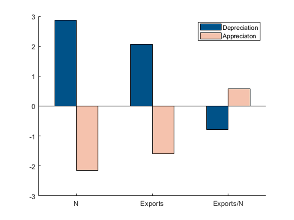
Percent change in exporter activity in period 1 with an expected 10 percent depreciation (solid blue bars) or appreciation (hollow orange bars) in period 2.
"Forward-guidance" for exchange rates?
In our model, we can also consider how information about the future exchange rate affects exporting activity in the second period. Suppose that that the exchange rate drops by 10 percent from the first to the second period. How different are total exports in the second period when firms expect the deprecation relative to when they do not? We find that when firms expect the depreciation, exports in the second period are higher because of two mechanisms. The first mechanism works through the extensive margin: An expected depreciation increases the stock of exporters in the first period, and most of these new exporters continue exporting in the second period, thereby increasing second-period exports. The second mechanism works through the intensive margin: Because prices are sticky, the first-period pricing decision is dynamic, and first-period export prices are increasing in the expected future exchange rate. Thus, if exporters expect a constant exchange rate, they will charge higher prices than if they expect a depreciation. The higher price gets carried into the second period, which decreases firm-level exports both because higher prices decrease foreign demand and because more firms will be unprofitable at the higher price and find it optimal to exit the market. In our calibration, exports in the second period are nearly 3 percent higher in the second period if firms expected the 10 percent depreciation than when the depreciation was a surprise. Thus, the model tells us that information about future exchange rates can affect both current and future economic activity, even when the actual path of exchange rates is identical.
References
Alessandria, George, Costas Arkolakis, and Kim J. Ruhl (2021a) "Firm Dynamics and Trade," Annual Review of Economics, 13 (1).
Alessandria, George, Horag Choi, and Kim J. Ruhl (2021b) "Trade adjustment dynamics and the welfare gains from trade," Journal of International Economics, 131, 103458.
Bernard, Andrew B. and J. Bradford Jensen (2004) "Why Some Firms Export," The Review of Economics and Statistics, 86 (2), 561–569.
Das, Sanghamitra, Mark J. Roberts, and James R. Tybout (2007) "Market Entry Costs, Producer Heterogeneity, and Export Dynamics," Econometrica, 75 (3), 837–873.
Fernandes, Ana M., Caroline Freund, and Martha Denisse Pierola (2016) "Exporter behavior, country size and stage of development: Evidence from the exporter dynamics database," Journal of Development Economics, 119 (C), 121–137.
Meese, Richard A and Kenneth Rogoff (1983) "Empirical exchange rate models of the seventies: Do they fit out of sample?" Journal of International Economics, 14 (1-2), 3–24.
Melitz, Marc J (2003) "The impact of trade on intra-industry reallocations and aggregate industry productivity," econometrica, 71 (6), 1695–1725.
Mix, Carter (2020) "Technology, Geography, and Trade over Time: The Dynamic Effects of Changing Trade Policy," International Finance Discussion Papers 1304, Board of Governors of the Federal Reserve System (U.S.).
Morales, Eduardo, Gloria Sheu, and Andrés Zahler (2019) "Extended Gravity," The Review of Economic Studies, 86 (6), 2668–2712.
Roberts, Mark J. and James R. Tybout (1997) "The Decision to Export in Colombia: An Empirical Model of Entry with Sunk Costs," The American Economic Review, 87 (4), 545–564.
A. Baseline specification with SDT FE
Table 3: Robustness check: Sector-Destination-Time Fixed Effects
| (1) | (2) | (3) | (4) | (5) | (6) | |
|---|---|---|---|---|---|---|
| VARIABLES | Exports | Exports | EM | EM | IM | IM |
| O-D Spot | 0.302 | 0.303 | 0.267** | 0.268** | 0.0345 | 0.0351 |
| (0.212) | (0.212) | (0.122) | (0.122) | (0.124) | (0.124) | |
| O-D Fcst. | 0.762** | 1.027*** | -0.265 | |||
| (0.326) | (0.25) | (0.218) | ||||
| O-D Fcst. App. | -0.607 | -0.961*** | 0.354 | |||
| (0.454) | (0.337) | (0.345) | ||||
| O-D Fcst. Dep. | 0.914** | 1.092*** | -0.177 | |||
| (0.43) | (0.247) | (0.361) | ||||
| Fixed Effects | OSD+SDT | OSD+SDT | OSD+SDT | OSD+SDT | OSD+SDT | OSD+SDT |
| Observations | 148,163 | 148,163 | 148,163 | 148,163 | 148,163 | 148,163 |
| R2 | 0.924 | 0.925 | 0.977 | 0.977 | 0.904 | 0.904 |
| Cluster | FX pair | FX pair | FX pair | FX pair | FX pair | FX pair |
Robust standard errors in parentheses. *** p<0.01, ** p<0.05, * p<0.1
Forecasted exchange rates are expressed in deviation from the spot exchange rate, as in table 1. EM stands for the Extensive Margin of trade (i.e. the number of exporters) while IM stands for the Intensive Margin of trade (i.e. the average exported volume per exporter). OSD stands for Origin-Sector-Destination FEs, and ST stands for Sector-Time FEs. An increase in any exchange-rate variable indicates a depreciation of the source currency, except for "O-D Fcst. Appreciation" where the variable is defined as taking positive values for appreciations.
B. Baseline specification using PPML
Table 4: Robustness check: Pseudo-Poisson Maximum Likelihood
| (1) | (2) | (3) | (4) | (5) | (6) | |
|---|---|---|---|---|---|---|
| VARIABLES | Exports | Exports | EM | EM | IM | IM |
| O-D Spot | 0.167 | 0.121 | 0.203*** | 0.211*** | -0.141 | -0.193 |
| (0.453) | (0.461) | (0.0783) | (0.0779) | (0.444) | (0.431) | |
| O-D Fcst. | -0.166 | 0.816*** | -2.101** | |||
| (1.023) | (0.247) | (0.994) | ||||
| O-D Fcst. App. | -2.229 | -0.499 | -0.353 | |||
| (2.351) | (0.346) | (1.246) | ||||
| O-D Fcst. Dep. | -1.699 | 1.021*** | -4.195** | |||
| (1.179) | (0.235) | (1.771) | ||||
| Controls: | ||||||
| Destination-Sector Demand | ✓ | ✓ | ✓ | ✓ | ✓ | ✓ |
| USD Spot | ✓ | ✓ | ✓ | ✓ | ✓ | ✓ |
| USD Fcst. | ✓ | ✓ | ✓ | ✓ | ✓ | ✓ |
| Fixed Effects | OSD+ST | OSD+ST | OSD+ST | OSD+ST | OSD+ST | OSD+ST |
| Observations | 201,046 | 201,046 | 261,234 | 261,234 | 201,046 | 201,046 |
| Pseudo R2 | 0.955 | 0.955 | 0.96 | 0.96 | 0.931 | 0.931 |
| Cluster | FX pair | FX pair | FX pair | FX pair | FX pair | FX pair |
Robust standard errors in parentheses. *** p<0.01, ** p<0.05, * p<0.1
Forecasted exchange rates are expressed in deviation from the spot exchange rate, as in table 1. EM stands for the Extensive Margin of trade (i.e. the number of exporters) while IM stands for the Intensive Margin of trade (i.e. the average exported volume per exporter). OSD stands for Origin-Sector-Destination FEs, and ST stands for Sector-Time FEs. An increase in any exchange-rate variable indicates a depreciation of the source currency, except for "O-D Fcst. Appreciation" where the variable is defined as taking positive values for appreciations.
1. Email: [email protected]. Return to text
2. Email: [email protected]. Return to text
3. Email: [email protected]. Return to text
4. Email: [email protected]. Return to text
5. See Fernandes et al. (2016). Due to data availability across different sources, our final sample covers the period 2006–2014. Return to text
6. Our results hold when using a Pseudo-Poisson Maximum Likelihood estimation which enables for the inclusion of country-pair-sector observations with zero trade flows and avoids inconsistent estimations as a consequence of the log-linearizing the error term. Our results also hold when including Sector-Destination-Time fixed effect to control for destination specific shocks. In such case, our Destination-Sector Demand proxy as well as USD related variables are dropped from the specification. These results can be found in appendix. Return to text
7. A demand curve of this kind arises naturally from a CES model with monopolistically competitive firms. See, for example, Melitz (2003). Return to text
8. Among others, see Bernard and Jensen (2004) and Alessandria et al. (2021b) Return to text
de Soyres, François, Erik Frohm, Emily Highkin, and Carter Mix. (2021). "Forward Looking Exporters," FEDS Notes. Washington: Board of Governors of the Federal Reserve System, October 6, 2021, https://doi.org/10.17016/2380-7172.2983.
Disclaimer: FEDS Notes are articles in which Board staff offer their own views and present analysis on a range of topics in economics and finance. These articles are shorter and less technically oriented than FEDS Working Papers and IFDP papers.