FEDS Notes
April 20, 2017
Job Reallocation and Unemployment in Equilibrium
Alison Weingarden1
1. Overview
Job reallocation in the U.S.– the sum of job creation and job destruction across employers– has been declining over several decades. According to the literature, the most plausible explanations rest on two trends: aging firms and aging workers.2 Older firms have lower rates of job creation and job destruction compared to younger firms or startups; similarly, older workers generally have longer job tenures compared to younger workers. Nevertheless, much of the decline in job reallocation remains unexplained. For example, Molloy et. al (2016) find a common secular decline in reallocation across many measures but conclude that the decline cannot be attributed to a single overarching cause.
Since the job reallocation process can change the rate at which workers enter and exit unemployment, it may also affect the rate of unemployment in steady state. However, the labor market consequences of declining reallocation are an open question; empirical evidence thus far is inconclusive.3
This piece looks at the relationship between job reallocation and the long-run rate of unemployment ("LRU") both theoretically and empirically. I define LRU as the average equilibrium (or steady-state) unemployment rate over several years or decades. Thus, my starting point is a widely-accepted formula for steady-state unemployment that uses two variables: the separation rate into unemployment and the job-finding rate out of unemployment. The separation rate is closely linked to job destruction, while the job-finding rate is closely linked to job creation. All else equal, less frequent separations reduce the LRU whereas less frequent job-finding increases the LRU. However, what happens to the LRU when separation and job-finding rates both decline? I show that theoretically, a decline in job reallocation has ambiguous relationship with the LRU. Empirically, it also appears that the decline in U.S. job reallocation had no impact on the LRU over a fairly long time horizon.
2. Theoretical framework
Previous literature has used a simple formula to relate worker flows to the steady-state unemployment rate (u*). In a search model with only two states -- employment and unemployment -- u* can be calculated by assuming that the number of workers flowing into unemployment equals the number flowing out. Thus, the steady-state unemployment rate is defined as, $$u^* = \frac{U^*}{U^*+E^*} = \frac{s}{s+f}$$ where the second equality indicates that steady-state values for E* and U* can be inferred from two structural parameters: the separation rate s and the job-finding rate f (s ≡ xs / E, the number of workers flowing from E to U divided by the stock of E; and f ≡ xf / U, a corresponding measure for U to E flows).4
A further step is needed to connect job reallocation to steady-state unemployment. Importantly, u* is calculated from rates of worker flows into and out of unemployment whereas job reallocation (JR) is the sum of job creation (JC) and job destruction (JD), both measured at the establishment level. As a result, the worker-based and job-based measures can differ. For example, since many job flows result from workers switching jobs (so-called E to E transitions), JC does not necessarily imply that a worker is hired from unemployment, nor does JD necessarily imply that a worker will enter into unemployment. Furthermore, gross churn (GC) -- when workers are replaced within an establishment but the establishment's headcount does not change -- are not counted in JR but they can increase the number of workers flowing into and out of unemployment.
Despite fundamental differences between worker and job flows, the two are closely related. The following equation expresses job reallocation in terms of worker flows into and out of unemployment (xs and xf, respectively): JR ≡ JC + JD = xs + xf + 2y − GC where y denotes job-to-job flows (E to E transitions).5 In steady state the expression simplifies to JR = 2x + 2y − GC, where x denotes both types of worker flows. Turning back to the expression for u*, clearly x does not affect u* because x is in the numerator of both s and f. It can also be shown that y and GC have no direct impact on the components of u* (detailed in the footnote below).6 Thus, perhaps unsurprisingly, this reveals an indeterminate relationship between JR and u*. Chart 1 below illustrates various combinations of JR and u* in four scenarios with different levels of job reallocation.
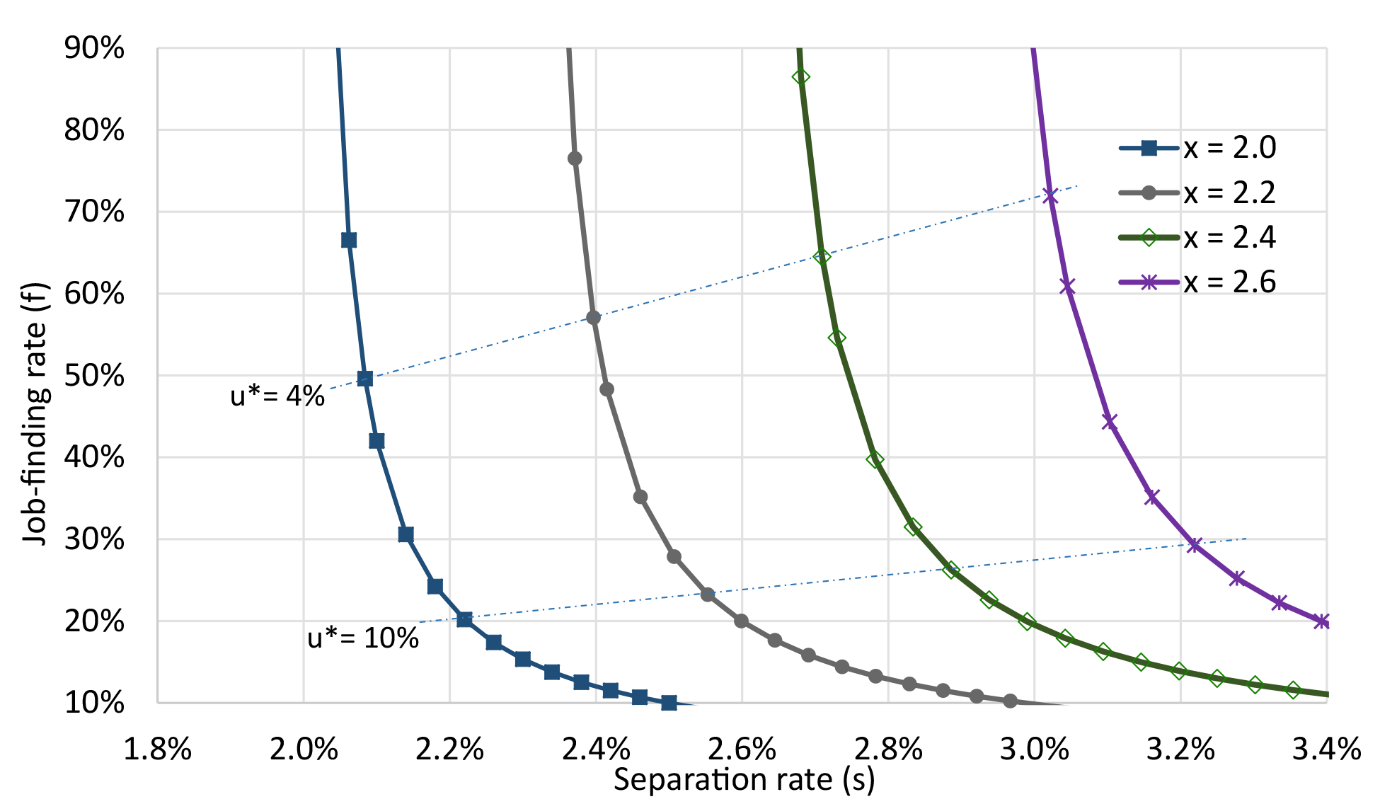
Note: I assume 2y = GC and U + E = 100 in all scenarios.
As the graph above shows, there are many possible values of u* for each level of x. If s and f both decline by the same proportion then u* is unchanged, whereas a decline in s alone lowers u* and a decline in f alone raises u*. Thus, a decline in aggregate job reallocation can correspond to a higher or lower LRU, depending on whether the fall in f is larger or smaller than the fall in s.7
3. Empirical analysis
This section investigates whether f and s have changed over time and what that might imply for the LRU. To begin the investigation, Chart 2 shows the result of applying the u* formula to high-frequency data from the Current Population Survey over the last five decades. When u* is calculated from monthly values of s and f, both the two-state and three-state models of u* closely match the observed unemployment rate.
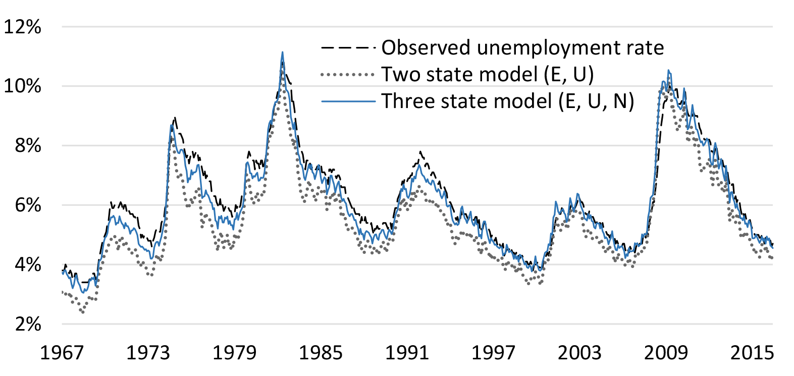
Source: Elsby et. al (2014) for historical transition rate data.8 From 1994 onward, calculations are based on the Current Population Survey, including the monthly Labor Force Status Flows data. The graph shows three-month centered moving averages.
Chart 2 illustrates that a meaningful calculation of the LRU requires estimates of the non-cyclical components of s and f, not just their monthly values. To infer longer trends in s and f, Chart 3 shows four points representing average rates of s and f over different time horizons within the last 50 years. The corresponding values in Table 1 illustrate these average rates of s and f, along with corresponding estimates of u*.
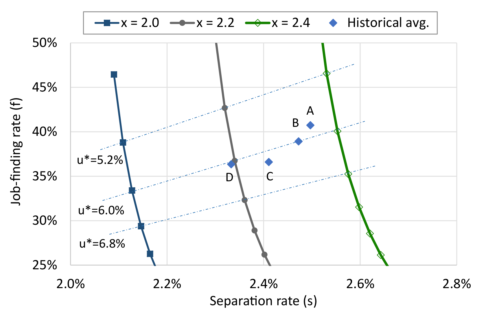
Source: Author’s calculations based on Current Population Survey data and historical data from Elsby et. al (2014). It is assumed that 2y = GC and U + E = 100 in all scenarios.
Table 1: Historical Averages of s and f and Estimated u*, 1967-2016
| Point | Number of years | Start | s | f | LRU |
|---|---|---|---|---|---|
| A | 50 | 1967 | 2.5% | 40.7% | 5.8% |
| B | 35 | 1982 | 2.5% | 38.9% | 6.0% |
| C | 15 | 2002 | 2.4% | 36.6% | 6.2% |
| D | 5 | 2012 | 2.3% | 36.3% | 6.0% |
Source: Author's calculations based on Current Population Survey data and historical data from Elsby et. al (2014). LRU is calculated from u*=s/(s+f) using average s and f, all based on a three-state model.
Interestingly, while s and f have both declined over time, these declines seem to have had minimal impacts on the estimated LRU; it is generally close to six percent in all cases.
4. Conclusion and discussion
In this piece I show how declines in job reallocation can coincide with higher or lower unemployment– the sign and magnitude of the relationship is ambiguous. Moreover, based on historical U.S. data, I find that the decline in job reallocation over the last several decades does not appear to have had much of an impact on the implied long-run rate of unemployment.
Although this piece has focused on the ways in which job reallocation might affect unemployment, there are other welfare issues related to job reallocation. For workers, declining reallocation may have benefits such as less frequent job searching and more accumulation of firm-specific human capital. However, low reallocation may have negative effects on workers such as stymied job ladders, long-duration unemployment, and matches that are lower in productivity or less preferred (along monetary or non-monetary dimensions). As discussed in Davis and Haltiwanger (2014), the impact of declining labor market dynamism on labor force participation is another important issue; low job-finding rates could marginalize a subset of particularly vulnerable workers– those with limited skills, the long-term unemployed, or young people who may not find jobs that allow them to build human capital. For producers, declining reallocation may reflect positive changes in firms' abilities to cope with shocks or it may reflect detrimental changes to the business environment such as high barriers to entry or large labor adjustment costs. While recent papers have explored many issues related to declining dynamism, there is ample space for future research.
Bibliography
Davis, Steven J., R. Jason Faberman, John Haltiwanger, Ron Jarmin, and Javier Miranda (2010). "Business Volatility, Job Destruction, and Unemployment." American Economic Journal: Macroeconomics, 2(2): 259-87.
Davis, Steven, and John Haltiwanger (2014). "Labor Market Fluidity and Economic Performance." Paper presented at the 2014 Federal Reserve Bank of Kansas City Economic Symposium Conference in Jackson Hole, WY.
Decker, Ryan, John Haltiwanger, Ron S. Jarmin, and Javier Miranda (2014). "The Role of Entrepreneurship in US Job Creation and Economic Dynamism," Journal of Economic Perspectives, 28(3), pp. 3-24.
Elsby, Michael W. L., Ryan Michaels, and David Ratner (2014). "The Beveridge Curve: A Survey," Journal of Economic Literature, 53(3), pp. 571-630.
Hyatt, Henry and James Spletzer (2013). "The Recent Decline in Employment Dynamics," IZA Journal of Labor Economics, 2(1), pp. 1-21.
Molloy, Raven, Christopher L. Smith, and Abigail Wozniak (2014). "Declining Migration Within the U.S.: The Role of the Labor Market," Finance and Economics Discussion Series 2013-27. Board of Governors of the Federal Reserve System.
Molloy, Raven, Christopher L. Smith, Riccardo Trezzi, and Abigail Wozniak (2016). "Understanding Declining Fluidity in the U.S. Labor Market," Finance and Economics Discussion Series 2016-15. Board of Governors of the Federal Reserve System.
U.S. Bureau of Labor Statistics. Current Population Survey, accessed January 2017, https://www.bls.gov/cps/
1. The author thanks Ryan Decker and Paolo Ramezzana for helpful comments on earlier drafts and David Ratner for advice and historical data. The idea for this note was prompted by discussions with Isabel Cairó and John Roberts. Return to text
2. Decker et. al (2014) focus on business dynamics while Hyatt and Spletzer (2013) and Molloy et. al (2014) focus on worker dynamics. Return to text
3. For instance, Davis et. al (2010) showed that declines in job destruction had a positive impact on labor markets through lower aggregate unemployment in the 1982–2005 period. In contrast, Davis and Haltiwanger (2014), which focuses on interstate differences in the 1998–2011 period, find that declining reallocation has a negative impact on labor markets in part because lower reallocation marginalizes a subset of workers. Return to text
4. A three-state model accounts for workers' intervening states of non-participation -- see Elsby et. al (2014) for a thorough discussion. In the analysis of historical data, I use a three-state model based on worker transition rates $$p[\cdot]$$ with $$ s = p[EU] + \frac{p[EN] \cdot p[NU]}{p[NE] + p[NU]}$$ and $$f = p[UE]+\frac{p[UN] \cdot p[NE]}{p[NE] + p[NU]},$$ where N denotes non-participation. Return to text
5. There are two underlying equations. The first is an identity for total hires, JC + ½GC = xf + y and the second is an identity for total separations, JD + ½GC = xs + y (following the literature, neither of these equations accounts for multiple job-holding by workers). Combining and rearranging yields JC + JD = xf + xs + 2y − GC. As an aside, when looking at the difference between job creation and job destruction, xf can proxy for JC and xs can proxy for JD. Return to text
6. Since y represents a job-to-job (or EE) flow, it should be clear that s and f are unaffected when a worker changes employer but remains employed. The argument that GC does not affect u* is more subtle. The hiring portion of gross churn may involve EE or UE flows and the separation portion may involve EE or EU flows. However, any UE or EU flows are reflected directly in xf and xs measures; therefore in equilibrium, GC should have no direct impact on the components of u*. Return to text
7. There may also be interactions between JR and short-term unemployment rate dynamics; these are outside the scope of this note. Return to text
8. Data prior to 1990 were tabulated by Joe Ritter and made available by Hoyt Bleakley. Return to text
Weingarden, Alison (2017). "Job Reallocation and Unemployment in Equilibrium," FEDS Notes. Washington: Board of Governors of the Federal Reserve System, April 20, 2017, https://doi.org/10.17016/2380-7172.1964.
Disclaimer: FEDS Notes are articles in which Board staff offer their own views and present analysis on a range of topics in economics and finance. These articles are shorter and less technically oriented than FEDS Working Papers and IFDP papers.