


FEDS Notes
July 31, 2026
Monetary Policy Stance and Commodity Cycles in Emerging Economies
Oscar Monterroso and Diego Vilán
Emerging market economies, particularly those that depend heavily on commodity exports, have long been characterized by more volatile and disruptive business-cycle dynamics than their advanced-economy counterparts. A large literature has studied the drivers of these fluctuations, including total factor productivity shocks, world interest rate shocks, and terms-of-trade disturbances. Within this literature, commodity price shocks have emerged as a central source of macroeconomic volatility. Because agricultural products, fuels, metals, and other primary commodities are traded in global markets, small open economies generally have little influence over their prices. Commodity-exporting emerging economies are therefore especially vulnerable to fluctuations in the prices of their key exports. Moreover, as emphasized by Drechsel et al (2026), recent geopolitical events—including the wars in Ukraine and the Middle East—as well as increasingly frequent climate-related shocks suggest that episodes of heightened commodity-market volatility are likely to remain a recurring feature of the global environment. This poses an important challenge for central banks in commodity-exporting emerging economies, which must gauge the appropriate monetary policy response to shocks that affect inflation, output, exchange rates, and financial conditions simultaneously.
In this note, we assess the trade-offs faced by the central bank of a commodity-exporting emerging economy, with particular emphasis on how commodity-price shocks affect the monetary-policy stance. The analysis proceeds in four steps. First, we summarize the relevant stylized facts and update the evidence on the negative co-movement between commodity prices and sovereign spreads by estimating two separate single-factor dynamic factor models for a sample of commodity-exporting emerging economies. Second, we incorporate two transmission channels into a small-open-economy semi-structural model: a direct income effect of export commodity prices on aggregate demand and a country-risk channel through which commodity prices affect sovereign spreads, the exchange rate, and the natural rate of interest. Third, we discipline these channels using country-specific regressions for a sample of commodity-exporting emerging economies. Finally, we study the model's impulse responses to a one-standard-deviation commodity-price shock and compare the baseline responses with counterfactual exercises that shut down or weaken the commodity-spread channel. The exercises show that the assessment of the monetary-policy stance depends critically on how these two channels interact. By compressing country-risk premia, higher commodity prices lower the natural real rate of interest and reinforce the appreciation of the currency. The decline in the natural real rate reduces the neutral nominal rate, while the currency appreciation dampens inflationary pressures. As a result, the monetary-policy stance can become more restrictive even when the policy rate is reduced.
Commodity prices and macroeconomic fluctuations
As emphasized by Drechsel and Tenreyro (2018), Shousha (2016), Fernández et al. (2018), and related work, several stylized facts characterize the relationship between business-cycle dynamics and commodity prices in emerging market economies. First, macroeconomic aggregates—including output, consumption, and investment—are typically more volatile in emerging market economies than in advanced economies. Second, commodity prices are positively associated with measures of real activity, such as output and investment. By contrast, the trade balance-to-GDP ratio and sovereign spreads tend to be countercyclical. Third, commodity prices tend to co-move negatively with country interest-rate spreads and are associated with a real appreciation of the currency. Fourth, evidence from structural VARs and theoretical models suggests that commodity-price shocks have stronger macroeconomic effects in emerging market economies than in advanced economies. In these frameworks, variance decompositions indicate that commodity-price shocks explain a significant fraction of fluctuations in output, consumption, and investment.
Motivated by these findings, most modeling frameworks share the same economic intuition about the transmission of commodity-price shocks. As suggested by Fernández et al. (2018), a positive commodity-price shock acts as an income shock that stimulates domestic demand. Higher demand for domestic goods raises their relative price and appreciates the country's real exchange rate. The increase in the relative price of domestic goods raises the expected profitability of domestic production and increases the marginal product of capital in that sector. This strengthens firms' demand for capital. Simultaneously, as the real appreciation makes non-commodity domestic goods relatively more expensive for foreign buyers and higher domestic absorption raises import demand, the trade balance tends to deteriorate.
Commodity Cycles and External Borrowing Costs
The income channel captures a central transmission mechanism through which commodity-price shocks can generate sizable fluctuations in output, investment, the real exchange rate, and the trade balance. However, for many commodity-exporting emerging economies, commodity prices may also affect the economy through a second channel: country risk spreads.1 Higher commodity prices can improve perceived repayment capacity, relax external financing constraints, and reduce the interest rate charged by foreign lenders. While the procyclical nature of commodity prices has been studied extensively, relatively less attention has been paid to the co-movement between commodity prices and country risk premia.
To this end, and in the spirit of Bastourre et al. (2012), we estimate two separate single-factor dynamic factor models (DFMs) over the period 2002Q1–2025Q4—one using commodity-price series and one using sovereign-spread series—for a sample of 13 emerging economies.2 In each model, the latent factor is assumed to follow an AR(2) process and summarizes the common component of the corresponding block of standardized series.3 Figure 1 plots the resulting commodity-price and sovereign-spread factors. In line with Bastourre et al. (2012) and Fernández et al. (2018), the estimated factors display strong negative co-movement: for the full sample, their correlation is -0.35.
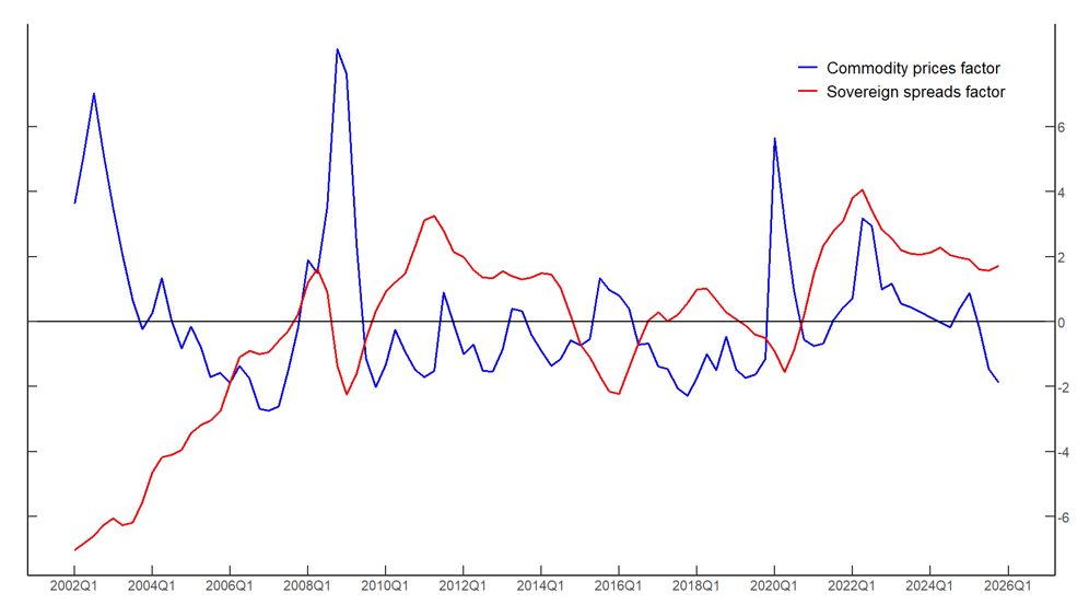
The commodity-price factor captures major developments in global commodity markets as documented by Kabundi and Zahid (2023) and related work. In particular, it captures the broad commodity boom-bust cycle of the 2000s. During this period, rapid growth in emerging and developing economies—especially China—contributed to a substantial increase in global commodity demand relative to the 1980s and 1990s. Over the period 2006–2008, prices for copper, crude oil, and wheat increased by 75 percent, 104 percent, and 110 percent, respectively. This synchronized surge was subsequently disrupted by the Global Financial Crisis, with prices falling back to early-2006 levels by the end of 2008. The sovereign-spread factor moves closely, and in the opposite direction, around this episode: the upswing in commodity prices beginning in 2006 was accompanied by a decline in sovereign spreads, while the Global Financial Crisis was followed by a sharp reversal in spreads that remained above their mean for several years. The analysis is also consistent with the broad decline in commodity prices observed in 2015—driven by global oil oversupply, weaker demand from China, and other factors—and with the surge in commodity prices during the rebound in economic activity following the COVID-19 pandemic.
Overall, the evidence suggests that country-risk dynamics are also closely linked to commodity cycles. Bastourre et al. (2012), Min et al. (2003), and related work argue that commodity prices are an important fundamental determinant of bond spreads for commodity-exporting economies. They also emphasize that common global forces can move commodity prices and sovereign spreads in opposite directions: declines in international interest rates, stronger global risk appetite, increases in global liquidity, higher equity returns, and U.S. dollar depreciations tend to support commodity prices while compressing sovereign spreads. At the country level, higher commodity prices can relax liquidity constraints, improve repayment capacity, and reduce the likelihood of debt-service and liquidity problems. These mechanisms help rationalize both the negative relationship between commodity prices and country risk premia observed in the data and, as highlighted by Uribe and Yue (2006), the role of country spreads in driving emerging-market business cycles and propagating foreign shocks.
A semi-structural approach
To assess the effects of commodity-price shocks on the monetary-policy stance, we employ a New Keynesian semi-structural model in the spirit of Ouliaris and Rochon (2026), Botha et al. (2017), Abradu-Otoo et al. (2024), and related work. The model incorporates real and nominal rigidities and assumes that monetary policy is neutral in the long run. It estimates trend or equilibrium components for key macroeconomic variables—such as potential output, trend inflation, the natural rate of interest, and the equilibrium real exchange rate—and computes deviations from these long-run benchmarks. In addition, we extend the standard framework by incorporating a block that captures the relationship between export commodity prices and a country's risk premium. The full model specification is outlined below.
The first block of the model is an aggregate-demand equation, or IS curve, in which the output gap $$(\hat{y}_t)$$ depends on its own persistence $$(\hat{y}_{t-1})$$, a monetary conditions index $$(mc i_t)$$, the foreign output gap $$(\hat{y}_t^{*})$$, the commodity export price index gap $$(\hat{q}_t^{com})$$, and an aggregate-demand shock $$(\epsilon_t^{\hat{y}})$$. The monetary conditions index summarizes the channels through which the real interest rate and the real exchange rate affect aggregate demand. It is defined as a weighted average of the real interest rate gap $$(\hat{r}_t)$$, measured as the deviation of the real interest rate from the natural rate of interest, and the real exchange rate gap $$(\hat{z}_t)$$, measured as the deviation of the real effective exchange rate from its trend level. We allow deviations of the commodity export price index from trend to affect the output gap directly, capturing the income effect of commodity-price fluctuations.
$$$$ \hat{y}_t = b_1\hat{y}_{t-1} - b_2 mc i_t + b_3\hat{y}_t^{*} + b_5\hat{q}_t^{com} + \epsilon_t^{\hat{y}} $$$$
$$$$ mci_t = b_4\hat{r}_t + (1-b_4)(-\hat{z}_t) $$$$
The second block is an inflation equation, or Phillips curve, in which inflation $$(\pi_t)$$ depends on its own persistence $$(\pi_{t-1})$$, inflation expectations $$(E_t\pi_{t+1})$$, real marginal costs $$(rmc_t)$$, and a cost-push shock $$(\epsilon_t^\pi)$$. Real marginal costs are modeled as a weighted average of the output gap, which captures the marginal costs of domestic producers, and the real exchange rate gap $$(\hat{z}_t)$$, which captures the marginal costs faced by importers.
$$$$ \pi_t=a_1\pi_{t-1}+\left(1-a_1\right)E_t\pi_{t+1}+a_2rmc_t+\epsilon_t^\pi $$$$
$$$$ rmc_t = a_3\hat{y}_t + (1-a_3)\hat{z}_t $$$$
The third block is an uncovered interest parity condition. The UIP condition relates the nominal exchange rate $$(s_t)$$ to its expected future value $$(E_ts_{t+1})$$, the differential between foreign $$(i_t^\ast)$$ and domestic nominal interest rates $$(i_t)$$, and a country risk premium $$(prem_t)$$. The exchange-rate equation also includes a backward-looking component, which allows the exchange rate to depend on past exchange-rate dynamics adjusted for trend real exchange rate depreciation and the average inflation differential. The nominal exchange rate is defined as units of domestic currency per unit of foreign currency, so that a decline in the nominal exchange rate corresponds to a nominal appreciation.
$$$$ s_t=\left(1-e_1\right)E_ts_{t+1}+e_1\left[s_{t-1}+\frac{2}{4}\left(\pi_t^T-{\bar{\pi}}_t^\ast+\mathrm{\Delta}{\bar{z}}_t\right)\right]+\frac{1}{4}\left(i_t^\ast-i_t+prem_t\right)+\epsilon^s $$$$
The monetary-policy block is described by a Taylor-type reaction function. The nominal policy interest rate depends on interest-rate persistence, the deviation of expected inflation $$(E_t \pi_{t+N}^4)$$ from the inflation target $$(\pi_{t+N}^T)$$, and the output gap:
$$$$ i_t = g_1 i_{t-1} + (1 - g_1)\{i_t^n + g_2[E_t \pi_{t+N}^4 - \pi_{t+N}^T] + g_3 \hat{y}_t\} + \epsilon_t^i $$$$
The variable $$(i_t^n)$$ represents the model's time-varying neutral nominal rate. This variable provides the nominal benchmark embedded in the policy rule and is constructed as the sum of the natural real interest rate, $$({\bar{r}}_t)$$, and expected year-on-year inflation $$(N)$$ quarters ahead:
$$$$ i_t^n={\bar{r}}_t+E_t\pi_{t+N}^4 $$$$
The policy rate generally differs from this benchmark because the central bank responds to deviations of expected inflation from target and to the output gap. In addition, the lagged policy-rate term introduces interest-rate smoothing, so the policy rate adjusts gradually over time. Thus, $$(i_t^n)$$ should be interpreted as the neutral nominal benchmark toward which the policy rule converges when expected inflation is at target, the output gap is closed, policy shocks are absent, and smoothing dynamics have dissipated. We define the monetary-policy stance (MPS) as the deviation of the nominal policy rate from its neutral level:
$$$$ {{MPS_t=\ i}_t-i}_t^n $$$$
A positive value indicates a restrictive stance, as the policy rate lies above its neutral level, while a negative value indicates an accommodative stance. Under this definition, the stance can become more restrictive even if the policy rate declines, provided that the neutral nominal interest rate falls by more.
The fourth block links export commodity prices and the country risk premium. Consistent with the small open-economy assumption, the economy is a price taker in global commodity markets. We therefore do not impose additional economic structure on the commodity export price index gap $$(\hat{q}_t^{com})$$ and instead assume that it follows an exogenous AR(1) process. The country risk premium $$(prem_t)$$ depends on its own persistence, the commodity export price index gap, and a premium shock $$(\epsilon_t^{prem})$$. Thus, in addition to the income effect of commodity prices on the output gap, the model allows commodity prices to affect the economy through a country-risk channel: higher commodity prices reduce the country risk premium. In the vein of Shousha (2016), Fernández et al. (2018) and Drechsel and Tenreyro (2018), our modeling framework embeds the negative relationship between the premium and commodity prices in a reduced-form fashion. However, as highlighted by Fernández et al. (2018) and Drechsel and Tenreyro (2018), modeling the risk premia using a reduced-form approach does not provide a complete formal rationalization of this relationship. This opens an avenue for a more complete model of the determination of fluctuations in country risk and their interaction with commodity prices.
$$$$ \hat{q}_t^{com} = \rho_{\hat{q}^{com}} \hat{q}_{t-1}^{com} + \epsilon_t^{\hat{q}^{com}}\ $$$$
$$$$ prem_t = \rho_{prem} prem_{t-1} - \phi_q \hat{q}_t^{com} + \epsilon_t^{prem}\ $$$$
Finally, the model also features a foreign block. All foreign variables are assumed to be exogenous, consistent with the small open-economy assumption. The foreign output gap, the foreign nominal interest rate, and the foreign trend real interest rate follow AR(1) processes that converge to their steady-state values. The model incorporates the risk premium explicitly through the commodity-price and country-risk block, while the trend real interest rate is pinned down by a long-run version of the UIP condition expressed in real terms.
$$$$ \mathrm{\Delta}{\bar{z}}_{t+1}={\bar{r}}_t-{\bar{r}}_t^\ast-prem_t $$$$
We calibrate the model to capture the characteristics of a small open economy in which commodity exports constitute a sizable share of total exports. To calibrate the elasticity of sovereign spreads to commodity prices, we follow the approach of Monterroso and Vilán (2025) and select a group of emerging economies based on their commodity export shares. For the commodity export price index, we use the IMF commodity export price index constructed using the methodology of Gruss and Kebhaj (2019).4 The index weights individual commodities according to their export shares in total commodity exports. We use the ICE BofA US Dollar Sovereign Index as a proxy for the country risk premium, while quarterly output data are sourced from the IMF's National Economic Accounts and Haver Analytics. We compute output and commodity-price gaps using the Hodrick-Prescott filter. The calibration exercise is based on a sample of 13 emerging economies.5
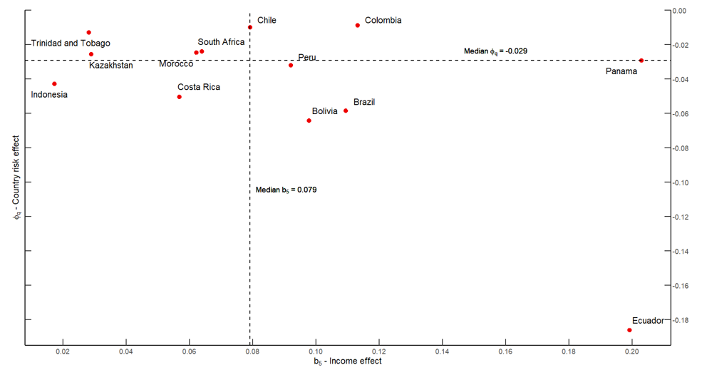
For the calibration of the income effect of commodity prices, we estimate country-specific regressions in which the output gap is regressed on a constant and the commodity export price index gap. The coefficient of interest captures the elasticity of the output gap with respect to commodity prices. For the calibration of the country-risk effect, we estimate country-specific regressions in which the country risk premium is regressed on a constant and the commodity export price index gap. The coefficient of interest captures the semi-elasticity of the country risk premium with respect to commodity prices.6
The evidence supports the presence of both income and country-risk effects. As Figure 2 shows, for the median country in the sample, the estimated income-effect coefficient is 0.079, while the estimated country-risk semi-elasticity is -0.029. Thus, higher commodity prices are associated with a wider output gap and a lower country risk premium. The full set of calibrated parameters and their descriptions is reported in Tables 1–3 in the Appendix.
Model dynamics and counterfactual exercise
We study the model's dynamics through the impulse responses to a one-standard-deviation commodity-price shock. Across the countries in the sample, the median standard deviation of the commodity-price-index gap is approximately 12 percent. Accordingly, we calibrate the commodity-price shock in the baseline scenario to this magnitude. We perform two exercises. First, we analyze the transmission of the shock under the baseline calibration. Second, we compare the baseline responses with a counterfactual specification in which the commodity-spread channel is shut down by setting the semi-elasticity of country spreads to commodity prices equal to zero.
Figure 3 reports the baseline impulse responses.7 On impact, the output gap rises, as the income effect induced by higher commodity prices leads to an expansion of domestic demand. The output gap remains positive for several quarters before gradually closing. The dynamics of inflation are governed by two opposing forces. On the one hand, above-normal demand raises marginal costs for domestic producers, putting upward pressure on inflation. On the other hand, higher commodity prices lead to an appreciation of the currency. This appreciation is reinforced by the effect of commodity prices on country risk spreads through the UIP condition. The appreciation lowers the domestic-currency cost of imported inputs, thereby mitigating the increase in firms' costs. As a result, inflation initially rises, mostly reflecting the expansion in the output gap. As the effect of the output gap begins to fade, inflation falls below its long-run level owing to the stronger real appreciation of the currency, with inflation persistence and expectations amplifying the decline. Finally, as the disinflationary pressures associated with the real exchange rate appreciation dissipate, inflation turns slightly positive again before converging back to steady state.
The joint dynamics of the output gap and the natural rate of interest present a challenging trade-off for the central bank. In line with Zhang et al. (2021), Zarazúa Juárez (2023), and related work, the decline in the country risk premium leads to a reduction in the natural rate of interest. In our baseline calibration, this effect amounts to about 50 basis points in the short run. Since expected inflation remains relatively stable, the neutral nominal interest rate declines by a similar magnitude. Thus, while the positive output gap exerts upward pressure on the policy rate through the Taylor rule, the decline in the neutral nominal interest rate works in the opposite direction. In our baseline calibration, the latter effect dominates: the decline in the neutral nominal interest rate more than offsets the central bank's response to the positive output gap. As a result, the central bank lowers the policy rate by about 20 basis points within four quarters of the shock. Overall, despite the reduction in the policy rate, the monetary-policy stance becomes more restrictive, as the policy-rate cut is not sufficient to offset the fall in the neutral nominal interest rate.
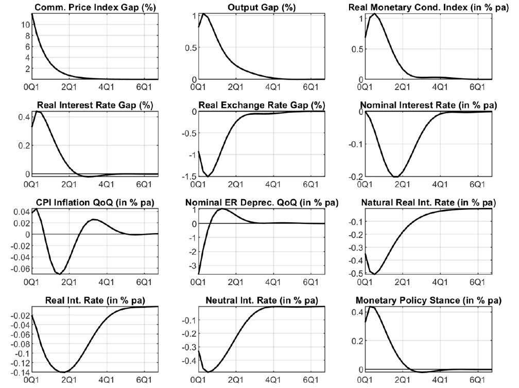
This tightening is also reflected in the real interest rate gap and the monetary conditions index. Although the real policy rate declines following the commodity-price shock, the natural rate of interest falls by more—approximately 50 basis points, compared with about 15 basis points for the real policy rate. Accordingly, the real interest rate gap turns positive. This, together with the strong real appreciation of the currency, leads to tighter monetary conditions, dampening aggregate demand and contributing to the gradual closing of the output gap.
Figure 4 compares the baseline responses with the counterfactual specification in which the commodity-spread channel is shut down. The response of the output gap is nearly identical across the baseline and counterfactual economies, reflecting the fact that both are subject to the same income effect from higher commodity prices. However, because higher commodity prices no longer compress the country's risk premium in the counterfactual, the nominal exchange rate appreciates by approximately 0.7 percentage points less on impact. This weaker appreciation attenuates the downward pressure on importers' real marginal costs and reduces the disinflationary pressures associated with the real appreciation of the currency. Consequently, inflation rises more on impact in the counterfactual specification than under the baseline calibration.
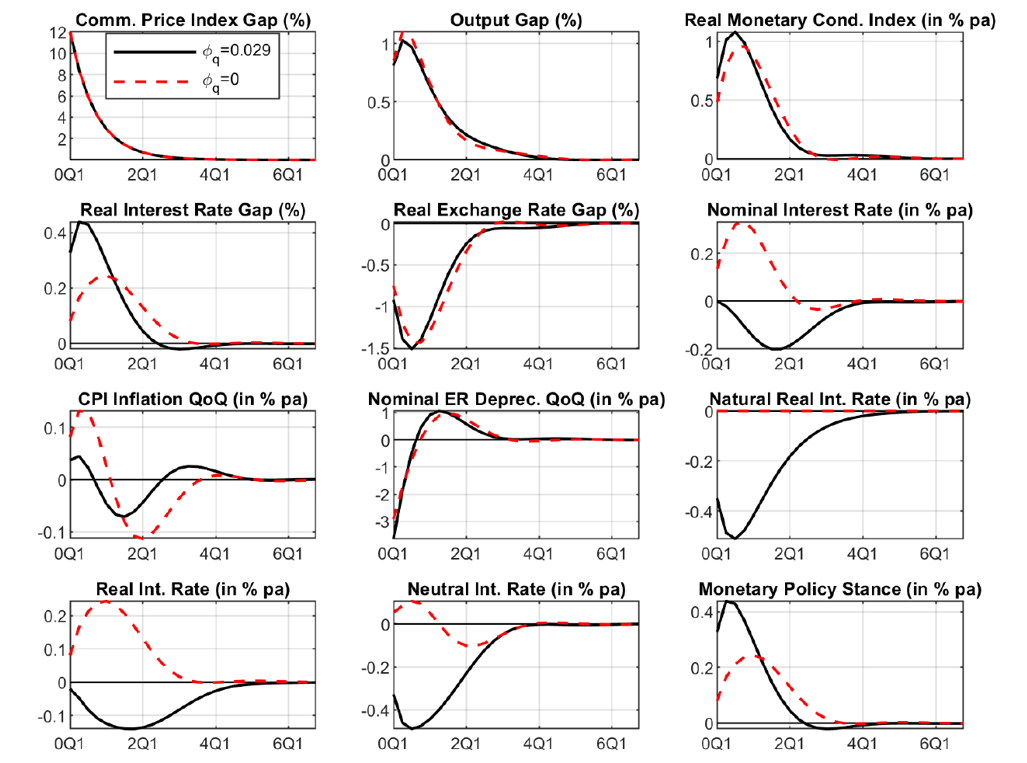
Shutting down the commodity-spread channel also has important implications for the response of the monetary authority. In the counterfactual exercise, the short-run spike in inflation triggered by the commodity-price shock is about 0.10 percentage points larger than under the baseline calibration. Although the subsequent undershooting of inflation is also larger, the economy no longer experiences the modest rebound of inflation above its long-run level documented in the baseline scenario. More importantly, because the country's risk premium is no longer compressed by higher commodity prices, the natural rate of interest does not respond to the shock, and the neutral nominal interest rate no longer declines. As a result, the challenging trade-off faced by the central bank in the baseline scenario—where the decline in the neutral nominal interest rate coincides with an increase in the output gap—is absent. Consequently, the central bank raises the policy rate by about 30 basis points, as prescribed by the Taylor rule.
These dynamics translate into a less restrictive monetary-policy stance relative to the baseline, since the neutral nominal interest rate is no longer depressed by the commodity-price shock. The policy-rate gap rises by around 25 basis points in the counterfactual, compared with more than 40 basis points under the baseline calibration. Unlike in the baseline calibration, the positive commodity-price shock triggers an increase in the real interest rate of more than 20 basis points, as the policy rate is no longer pulled down by a decline in the natural rate of interest. As a result, the real interest rate deviates less from its natural level, implying a smaller real interest rate gap and easing the tightening pressures associated with the interest-rate channel. Nevertheless, monetary conditions follow a broadly similar path, suggesting that the tightening in monetary conditions following a commodity-price shock is driven primarily by the real appreciation of the currency. Without the commodity-spread channel, however, the model predicts a slower adjustment of the policy rate, which takes more than a year to return to its pre-shock level.
Alternative calibrations
To provide some perspective, we compare our results with those of other relevant studies. The dependence of country risk premia, or interest-rate spreads, on commodity-price fluctuations is a key mechanism explored in related work, including Shousha (2016), Fernández et al. (2018), Drechsel and Tenreyro (2018), and Drechsel et al. (2026). In Shousha (2016), the interest rate is assumed to depend on the level of the real commodity export price index relative to its steady-state value, and the posterior mean of the parameter of interest for a sample of emerging economies is reported to be around -0.014. Fernández et al. (2018), in an extension of their benchmark framework, allow the process for country risk premia to depend on country fundamentals, including TFP and commodity prices. Their model is estimated for a group of emerging economies, with a median estimate of the relevant parameter equal to -0.008. In a similar vein, Drechsel and Tenreyro (2018) and Drechsel et al. (2026) use a semi-elasticity of interest-rate spreads with respect to export commodity prices of roughly -0.2.
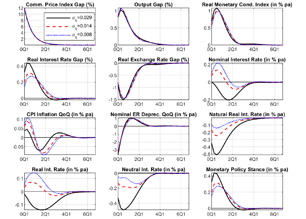
Figure 5 shows the model's impulse responses to a one-standard-deviation commodity-price shock under three alternative calibrations of the commodity-spread semi-elasticity: our baseline value and the closest comparable estimates from Shousha (2016) and Fernández et al. (2018). Relative to the baseline calibration, inflation rises by approximately 0.05 and 0.08 percentage points more in the short run under the calibrations of Shousha (2016) and Fernández et al. (2018), respectively. The results indicate that the calibration of the country-risk channel is crucial for the adjustment of the policy interest rate. As the sensitivity of the risk premium to commodity prices declines in absolute value, the natural rate of interest falls by less, exerting less downward pressure on the neutral nominal interest rate. Under the calibrations of Shousha (2016) and Fernández et al. (2018), the Taylor rule prescribes policy-rate increases of about 13 and 21 basis points, respectively. In addition, the monetary-policy stance becomes less restrictive than under the baseline calibration: the policy-rate gap rises to about 30 and 27 basis points, respectively, compared with approximately 42 basis points in the baseline calibration.
Overall, the exercise shows that the calibration of the commodity-spread semi-elasticity has quantitatively important implications for the conduct of monetary policy. A weaker commodity-spread channel attenuates the decline in the natural rate of interest and therefore reduces the downward pressure on the neutral nominal interest rate. As a result, the central bank responds more strongly to the inflationary and demand effects of the commodity-price shock, while the overall monetary-policy stance becomes less restrictive than under the baseline calibration.
Conclusions
In this note, we assess how a commodity-price shock affects the monetary-policy stance in a commodity-exporting emerging economy under an inflation-targeting regime and free capital mobility. Motivated by the procyclical nature of commodity prices and the negative co-movement between commodity prices and sovereign spreads documented in the literature, we emphasize two key channels through which commodity-price shocks propagate through the economy: an income channel and a country-risk channel. In our simulations, a positive commodity-price shock leads to a more restrictive monetary-policy stance, although the policy-rate response depends importantly on the extent to which the shock lowers the natural rate of interest. In particular, the stronger the compression in country risk premia, the larger the decline in the natural rate and the greater the downward pressure on the neutral nominal interest rate. Our counterfactual exercises show that the policy-rate path and the overall monetary-policy stance depend critically on the central bank's assessment of the country-risk channel, especially the sensitivity of country spreads to fluctuations in commodity prices. These findings, together with related work in the literature, underscore the need for further research on the determinants of country risk premia and their interaction with commodity prices in emerging market economies.
References
Abradu-Otoo, P., Acquah, J. K., Attuquaye, J., Harvey, S. K., Loloh, F., Mkhatrishvili, S., . . . Quansah, M. (2024, November). Quarterly Projection Model for the Bank of Ghana: Extensions and Applications (PDF). Retrieved from IMF Working Papers.
Bastourre, D., Carrera , J., Ibarlucia, J., & Sardi, M. (2012, October). Common Drivers in Emerging Market Spreads and Commodity Prices (PDF). Retrieved from Banco Central de la República Argentina.
Benes, J., Clinton , K., George, A., Gupta, P., John, J., Kamenik, O., . . . Zhang, F. (2017, February). Quarterly Projection Model of India: Key Elements and Properties (PDF). Retrieved from IMF Working Papers.
Botha, B., de Jager, S., Ruch, F., & Steinbach, R. (2017, September). The Quarterly Projection Model of the SARB (PDF). Retrieved from South African Reserve Bank Working Paper Series.
Drechsel , T., McLeay, M., Tenreyro , S., & Turri, E. D. (2026, May). How Should Central Banks Respond to Commodity Price Shocks? Optimal Monetary and Exchange Rate Frameworks for Commodity-Exposed Economies (PDF). Retrieved from NBER Working Paper Series.
Drechsel, T., & Tenreyro, S. (2018). Commodity booms and busts in emerging economies. Journal of International Economics, 200-218.
Fernández , A., González , A., & Rodríguez, D. (2018). Sharing a ride on the commodities roller coaster: Common factors in business cycles of emerging economies. Journal of International Economics, 99-121.
Gruss, B., & Kebhaj, S. (2019, January 24). Commodity Terms of Trade: A New Database. Retrieved from IMF Working Papers.
International Monetary Fund. (2015, October). World Economic Outlook (PDF). Adjusting to Lower Commodity Prices.
Kabundi, A., & Zahid, H. (2023, April). Commodity Price Cycles. Commonalities, Heterogeneities, and Drivers (PDF). Retrieved from Policy Research Working Paper. World Bank Group.
Min, H.-G., Lee, D.-H., Nam, C., Park, M.-C., & Nam, S.-H. (2003). Determinants of emerging-market bond spreads: Cross-country evidence. Global Financial Journal.
Monterroso, O., & Vilán, D. (2025, July 07). Commodity terms of trade uncertainty and economic activity in emerging economies. Retrieved from FEDS Notes.
Ouliaris, S., & Rochon, C. (2026, April 06). Solving the Canonical Quarterly Projection Model Using EViews. Retrieved from International Monetary Fund.
Shousha, S. (2016, January 25). Macroeconomic Effects of Commodity Booms and Busts: The Role of Financial Frictions (PDF).
Tenreyro, S., Drechsel, T., & McLeay, M. (2019, October 7). CEPR Discussion Paper. Retrieved from https://papers.ssrn.com/sol3/papers.cfm?abstract_id=3464575.
Uribe, M., & Yue, V. Z. (2006). Country spreads and emerging countries: Who drives whom? Journal of International Economics, 6-36.
World Bank Group. (2021, April). Commodity Markets Outlook (PDF). Causes and Consequences of Metal Price Shocks.
Zarazúa Juárez, C. A. (2023). Understanding the natural rate of interest for a small open economy. Latin American Journal of Central Banking.
Zhang, R., Martínez-García, E., Wynne, M. A., & Grossman, V. (2021). Ties that bind: Estimating the natural rate of interest for small open economies. Journal of International Money and Finance.
Appendix
Table 1. Model Calibration
| Parameter | Label | Value | Explanation |
|---|---|---|---|
| IS curve | |||
| Persistence | $$ b_1 $$ | 0.7 | Output persistence. Varies between 0.1 (extremely flexible) and 0.95 (extremely inflexible). |
| Interest rate channel | $$ b_2 $$ | 0.2 | Impact of monetary conditions on output gap. Varies between 0.1 (low impact) to 0.5 (strong impact). |
| External demand | $$ b_3 $$ | 0.5 | Impact of external demand on output gap. Varies between 0.1 and 0.7. |
| Weight of real rate gap in MCI | $$ b_4 $$ | 0.4 | Share of real rate in monetary conditions index. Varies between 0.3 and 0.8. |
| Weight of the commodity price index gap | $$ b_5 $$ | 0.079 | Median from calibration exercise in which the output gap is regressed on the commodity price index gap for 13 countries. |
| Phillips curve | |||
| Persistence | $$ a_1 $$ | 0.7 | Inflation persistence, which varies between 0.4 (low persistence) and 0.9 (high persistence). While a1 indicates the share of firms which exhibit backward-looking behavior when resetting prices, (1 −a1) is the share of forward-looking firms. |
| Pass-through of marginal costs to inflation | $$ a_2 $$ | 0.2 | Impact of real marginal costs on inflation. Varies between 0.1 (a flat Phillips curve and a high sacrifice ratio) and 0.5 (a steep Phillips curve and a low sacrifice ratio). |
| Ratio of domestic costs in firms' aggregate costs | $$ a_3 $$ | 0.6 | Varies between 0.9 (for a relatively more closed economy) to 0.5 (for a relatively more open economy). |
| Exchange rate | |||
| Persistence | $$ e_1 $$ | 0.4 | Nominal exchange rate persistence. Setting it equal to 0 reduces the equation to a simple UIP condition. |
| Policy rule | |||
| Interest rate smoothing | $$ g_1 $$ | 0.75 | Policy rate persistence. Varies from 0 (no persistence) to 0.8 ("wait-and-see" policy) |
| Weight on inflation deviation | $$ g_2 $$ | 1.5 | Response of the policy rate to expected inflation relative to target. The conventional Taylor Principle requires g2>1. |
| Weight on output gap | $$ g_3 $$ | 0.4 | Response of the policy rate to the output gap. A positive value implies policy tightening when the output gap is positive. |
| Commodity and premium blocks | |||
| Persistence of commodity price index gap | $$ \rho_\hat{q}{com} $$ | 0.7 | Persistence of AR(1) process for global commodity prices index gap |
| Persistence of premium | $$ \rho_{prem} $$ | 0.7 | Persistence of AR(1) process for the premium. |
| Pass-through of commodity prices to premium | $$ \phi_q $$ | 0.029 | Median on calibration exercise in which the premium is regressed on the commodity price index gap for 13 countries. |
Table 2. Model Calibration
| Parameter | Label | Value | Explanation |
|---|---|---|---|
| Steady state parameters | |||
| Potential output growth | $$\mathrm{\Delta}{\bar{y}}^{ss}$$ | 3 | Typically, an average over a relevant recent history. For advanced economies often around 2, for emerging economies would be typically higher (between 2 and 5). |
| Domestic inflation target | $${\bar{\pi}}^{ss}$$ | 4 | Based on announced or internal/informal inflation objective. |
| Domestic real interest rate | $${\bar{r}}^{ss}$$ | 0.5 | For advanced economies the value would be somewhere between 0.5 and 2. For emerging economies it can be higher due to higher required returns on capital. |
| Trend RER depreciation | $$\mathrm{\Delta}{\bar{z}}^{ss}$$ | -1.5 | It is typically 0 for advanced economies vs. other advanced economies. For emerging economies vs. advanced economies, it is typically negative (i.e., appreciation in the steady state) due to productivity and price convergence. |
| Foreign inflation target | $${\bar{\pi}}^{\ast s s}$$ | 2 | Long-run inflation rate in the foreign block, calibrated at 2 percent to represent the inflation objective of a typical advanced-economy trading partner. |
| Level of foreign real interest rate | $${\bar{r}}^{\ast s s}$$ | 0.75 | Representative long-run real interest rate for the advanced-economy foreign block, calibrated within a consistent with estimates for advanced economies. |
| Trends. Speed of convergence | |||
| Persistence of inflation target | $$\rho_{{\bar{\pi}}^T}$$ | 0.5 | Persistence of inflation target adjustment to the medium-term target. |
| Persistence of trend real exchange rate depreciation | $$\rho_{\mathrm{\Delta}\bar{z}}$$ | 0.8 | Persistence of AR(1) process for the trend real exchange rate depreciation |
| Persistence of trend output growth | $$\rho_{\mathrm{\Delta}\bar{y}}$$ | 0.8 | Persistence of AR(1) process for trend output growth. |
| Persistence of trend real interest rate | $$\rho_{\bar{r}}$$ | 0.8 | Persistence of AR(1) process for trend real interest rate. |
| Persistence of trend foreign real interest rate | $$\rho_{{\bar{r}}^\ast}$$ | 0.8 | Persistence of AR(1) process for the trend foreign real interest rate |
| Persistence in foreign output gap | $$\rho_{y^\ast}$$ | 0.8 | Persistence of AR(1) process for the foreign output gap |
| Persistence in foreign interest rates | $$\rho_{i^\ast}$$ | 0.8 | Persistence of AR(1) process for the foreign trend real interest rate. |
| Persistence in foreign inflation | $$\rho_{\pi^\ast}$$ | 0.8 | Persistence of AR(1) process for foreign trend inflation rate. |
Table 3. Model Calibration
| Parameter | Label | Value | Explanation |
|---|---|---|---|
| Standard deviations of shocks | |||
| Output gap shock | $$\sigma_\hat{y}$$ | 1 | Standard deviation of the shock in the IS curve |
| Cost-push (inflation shock) | $$\sigma_\pi$$ | 0.75 | Standard deviation of the shock in the Phillips curve |
| Monetary policy (interest rate) shock | $$\sigma_i$$ | 1 | Standard deviation of the shock in the monetary policy reaction function |
| UIP shock | $$\sigma_s$$ | 3 | Standard deviation of the shock in the UIP condition |
| Potential output growth shock | $$\sigma_{\mathrm{\Delta}\bar{y}}$$ | 0.5 | Standard deviation of the shock in the AR(1) process for trend output growth |
| Trend RER depreciation shock | $$\sigma_{\mathrm{\Delta}\bar{z}}$$ | 0.5 | Standard deviation of the shock in the AR(1) process for the trend RER depreciation |
| Trend real interest rate shock | $$\sigma_{\bar{r}}$$ | 0.5 | Standard deviation of the shock in the AR(1) process for the trend real interest rate |
| Inflation target shock | $$\sigma_{\pi^T}$$ | 2 | Standard deviation of the shock in the AR(1) process for the inflation target |
| Foreign output shock | $$\sigma_{{\bar{y}}^\ast}$$ | 1 | Standard deviation of the shock in the AR(1) process for the foreign output gap |
| Foreign interest rate shock | $$ \sigma_{i^\ast} $$ | 1 | Standard deviation of the shock in the AR(1) process for the foreign nominal interest rate |
| Foreign inflation shock | $$ \sigma_{\pi^\ast}$$ | 2 | Standard deviation of the shock in the AR(1) process for the foreign inflation rate |
| Foreign real interest rate shock | $$ \sigma_{{\bar{r}}^\ast} $$ | 0.5 | Standard deviation of the shock in the AR(1) process for the foreign real interest rate |
| Commodity price index gap shock | $$ \sigma_\hat{q}com $$ | 2 | Standard deviation of the shock in the AR(1) process for the commodity price index gap |
| Premium gap shock | $$ \sigma_\hat{prem} $$ | 1 | Standard deviation of the shock in the premium gap equation |
1. We define the country risk spread as the difference between the yield on a country's sovereign debt and the yield on a comparable risk-free benchmark. Return to text
2. The sample of 13 emerging economies corresponds to a geographically diverse sample of emerging economies which have a large share of commodity exports including: Trinidad and Tobago, Kazakhstan, Bolivia, Indonesia, Chile, Colombia, Ecuador, South Africa, Peru, Morocco, Brazil, Costa Rica and Panama. This sample is also used for the calibration of the model described in the next section. The estimation of the factor models is done via Maximum Likelihood methods. Return to text
3. Due to the high variability of the data, we standardize all series before estimating the DFMs. Each series is therefore expressed in standard deviations from its own mean. We also orient each estimated factor so that it is positively correlated with the cross-sectional average of the corresponding standardized series. Return to text
4. Gruss and Kebhaj (2019) provide a comprehensive database of country-specific commodity price indices for 182 economies since 1962. The database includes a commodity terms-of-trade index—which proxies the windfall gains and losses of income associated with changes in world prices—as well as additional country-specific series, including commodity export and import price indices. Return to text
5. For all sampled economies we employ quarterly data on output, the commodity export price index and the risk premium. Return to text
6. Regression samples are country-specific and depend on data availability. Return to text
7. Throughout the analysis, we focus on the conduct of conventional interest-rate policy under an inflation-targeting regime. We abstract from the use of other instruments that may also be employed by emerging-market central banks—such as foreign-exchange intervention, capital flow management measures, or macroprudential policies—in order to isolate the role of the conventional policy rate. Return to text
Monterroso, Oscar, and Diego Vilán (2026). "Monetary Policy Stance and Commodity Cycles in Emerging Economies," FEDS Notes. Washington: Board of Governors of the Federal Reserve System, July 31, 2026, https://doi.org/10.17016/2380-7172.4116.
Disclaimer: FEDS Notes are articles in which Board staff offer their own views and present analysis on a range of topics in economics and finance. These articles are shorter and less technically oriented than FEDS Working Papers and IFDP papers.