FEDS Notes
March 07, 2019
A New Procedure for Generating the Stochastic Simulations in FRB/US1
Manuel González-Astudillo and Diego Vilán
Introduction
This note summarizes a new procedure for generating stochastic simulations in FRB/US, a large-scale estimated general equilibrium macroeconomic model of the U.S. economy, which has been in use at the Federal Reserve Board since 1996.2 The new methodology addresses longstanding concerns about the capacity of the stochastic simulations in the FRB/US model to replicate certain features of the business cycle; in particular, the depth, duration, and frequency of the simulated recessions could often seem to be at odds with the data.
The original procedure to generate stochastic simulations in FRB/US was based on a bootstrap approach in which the errors were assumed to be independent across time. The residuals from relevant equations were drawn randomly with replacement and then applied to the model to obtain simulated trajectories of the variables into the future. The procedure therefore captured the correlation across equations in any given period, but not across time.
In contrast, the proposed new methodology introduces a Markov-switching approach featuring three main features. First, the transition from non-recession to recession periods is consistent with the transitions observed in the data. Second, recession periods are divided into two kinds, with one kind representing usual recessions and one kind representing the Great Recession. Third, once the simulated economy falls in a recession, the residuals from that recession are drawn in the same sequence as they occurred in the data, and then the simulated economy exits to the non-recession period deterministically.
We find that the typical recession generated by the original bootstrapping procedure is substantially shallower than that in the data. For example, the median peak-to-trough increase of the unemployment rate in the original approach is 1.8 percentage points, whereas it is 2.2 percentage points in the data. Furthermore, simulated recessions tend to be slightly shorter and less frequent than in the data. Under the new approach, the median simulated peak-to-trough increase of the unemployment rate is 2.1 percentage points and recession episodes tend to be more frequent than in the original simulation procedure. Looking beyond the median, the methodology described in this note generates a smaller proportion of mild recessions and a larger proportion of severe recessions.
In the first part of this note, we contrast some features of the original stochastic simulations procedure with those of the data. In the second part, we offer an alternative to the original procedure that fits the data better along core dimensions of interest.
- The original procedure for generating stochastic simulations using FRB/US
The original procedure--referred to interchangeably as the standard bootstrap or original procedure hereafter--samples residuals from 71 equations of the FRB/US model, including private spending, labor, price, fiscal, and financial variables from the 196 quarters covering 1969:Q1 through 2017:Q4.3 In each simulated period, a vector of these 71 equation residuals is drawn randomly in an independent manner with replacement and applied to a linearized version of the FRB/US model. This process is repeated for 20 quarters (5 years), which constitutes one model simulation. The model simulation is then repeated 20,000 times to obtain confidence intervals for real GDP growth, the unemployment rate, the core inflation rate, and the federal funds rate over the extended forecast horizon, as well as the probability of certain events.4 All simulations assumed an inertial version of the Taylor rule constrained by the effective lower bound (ELB).
- Evaluating the performance of the original stochastic simulation procedure
To evaluate the performance of the standard bootstrap, we simulate the linearized version of the FRB/US model around a baseline that is consistent with the median values for core macro variables from the Survey of Economic Projections (SEP) and compare its statistics with those of the historical data. We focus on the three following dimensions:
- The depth of recessions as measured by the peak-to-trough increase in the unemployment rate.
- The duration of recessions as measured by the length of peak-to-trough episodes.
- The frequency of recessions as measured by the number of recession episodes.
We focus mainly on recession episodes, as the initial source of concern was the model's ability to capture the distribution of severe adverse events seen in the data.
The model is simulated 20,000 times around a baseline in which the economy is roughly in steady state for 260 quarters by drawing residuals and discarding the initial 60 quarters to eliminate the effects of initial conditions.5 The simulations end up having 200 quarters each, roughly consistent with the 196 quarters between 1969:Q1 and 2017:Q4 from which we sample the model's residuals. That period is also the one from which we obtain the features of recessions in the data. Lastly, because we want to compare the model's recessions with those observed in the data, for most of which the ELB for the federal funds rate was not binding, we do not impose the ELB in the simulations.6
In order to compare the statistics from the simulations with the data, we need a definition of a recession in quarterly data that will allow us to discern when recessions in the model occur. As no formulaic procedure for dating a recession as used by the National Bureau of Economic Research (NBER) is available, we define a recession as an event in which there are four or more consecutive quarters of an increase in the unemployment rate and at least two quarters, not necessarily consecutive, of declining real GDP.7 Figure 1 shows that this alternative definition of recession--referred to as a recession proxy hereafter--coincides relatively closely with the official NBER recession dating since 1969.
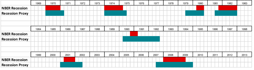
Table 1 compares the peak-to-trough statistics from the NBER recessions--where the peak and trough quarters are defined by that institution--with the statistics from the proxy recessions, where the peak is the quarter before the unemployment rate starts to increase and the trough is the quarter just before the unemployment rate begins to decline. Statistics for the unemployment rate, the core PCE price inflation rate, and the federal funds rate are shown. The lower panel of the table displays the length and frequency of recessions.
As can be seen, the peak-to-trough measures in the recession proxy periods are qualitatively very similar to those of the NBER recession periods. Specifically, in both cases, the median peak-to-trough increase in the unemployment rate is 2.2 percentage points. In what follows, we will use this statistic as our measure of the depth of recessions in the data. Additionally, as may be inferred from Figure 1, the proxy measure of recessions tends to be longer than NBER recessions--6 versus 4 quarters--and equally frequent--7 recession episodes in each case. These two statistics, namely the median length and frequency of recessions, will be our targets for these measures in the data. In sum, our mechanical definition of recessions, which we need to conduct the simulations, appears to work relatively well, in that the properties of the periods it identifies are quite close to the properties of the recessions identified by the NBER.
Table 1: Features of NBER and Proxy Recessions
Statistics for peak-to-trough changes during recessions in the data
| Variable | Statistic | NBER Recession | Recession Proxy |
|---|---|---|---|
| Unemployment rate (pp) | median | 2.2 | 2.2 |
| min | 0.9 | 1.5 | |
| max | 4.5 | 5.1 | |
| Core PCE inflation rate (pp) | median | -0.8 | -0.3 |
| min | -2.7 | -3.1 | |
| max | 5.2 | 6.0 | |
| Federal funds rate (pp) | median | -3.7 | -4.8 |
| min | -8.3 | -5.6 | |
| max | -1.7 | 2.6 |
Duration and frequency of recessions in the data
| Statistic | NBER Recession | Recession Proxy | |
|---|---|---|---|
| Length (quarters) | median | 4 | 6 |
| min | 2 | 5 | |
| max | 6 | 10 | |
| Frequency (episodes) | 7 | 7 |
2.1 How does the standard bootstrap perform?
The results of the simulations under the standard bootstrap conducted as described in Section 1 can be found in Table 2. In terms of medians, the model generates recessions that are not as deep as seen in the data. The peak-to-trough increase in the unemployment rate is 1.8 percentage points, compared with 2.2 percentage points in the data, and the change at the 90th percentile in the simulations is 2 percentage points below the maximum peak-to-trough increase observed in the data. Furthermore, the model creates proxy recessions that are slightly shorter and less frequent than is observed in the data. Nevertheless, the 90th percentile of the length of simulated recessions is large enough to cover the median length observed in history. The same is true for the 90th percentile of the frequency of recession episodes, which just covers the frequency of a recession in the data. All these features taken together raise serious concerns about the ability of the original stochastic simulation procedure to generate recessions that resemble their historical counterparts.
Table 2: Features of the standard bootstrap simulation method
Statistics for peak-to-trough changes during proxy recessions
| Variable | Statistic | Data | Model |
|---|---|---|---|
| Unemployment rate (pp) | median | 2.2 | 1.8 |
| 10th | 0.9 | ||
| 90th | 3.1 | ||
| Core PCE inflation rate (pp) | median | -0.3 | 0.0 |
| 10th | -1.3 | ||
| 90th | 1.4 | ||
| Federal funds rate (pp) | median | -4.8 | -1.1 |
| 10th | -3.1 | ||
| 90th | 0.4 |
Duration and frequency of proxy recessions
| Statistic | Data | Model | |
|---|---|---|---|
| Length (quarters) | median | 6 | 5 |
| 10th | 4 | ||
| 90th | 9 | ||
| Frequency (episodes) | median | 7* | 5 |
| 10th | 3 | ||
| 90th | 7 |
* Corresponds to the number of recession episodes in the data. Return to table
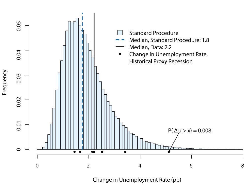
Figure 2 shows the frequency distribution of peak-to-trough increases in the unemployment rate during the proxy recessions obtained from the stochastic simulations. For comparison, Figure 2 also shows the observed peak-to-trough increases in the unemployment rate for the seven proxy recession episodes in history, indicated by black dots along the x-axis. The proxy recession episodes in our stochastic simulations are skewed heavily to the right, with five out of the seven historical events located to the right of the median from the simulations (the light blue vertical line). Moreover, the probability that a recession generated from the stochastic simulation is as extreme, or worse, as that observed during the Great Recession--the right-most black dot along the x-axis--is less than 1 percent, which we judge to be too low.
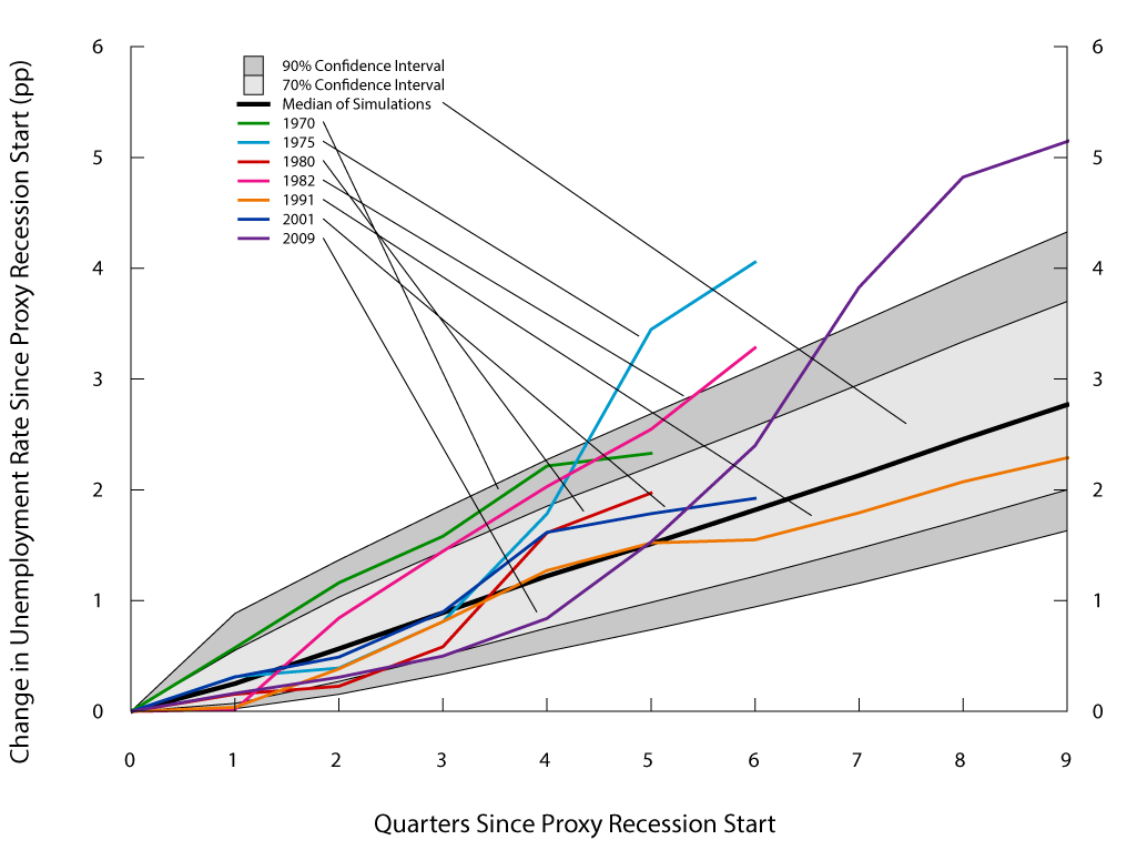
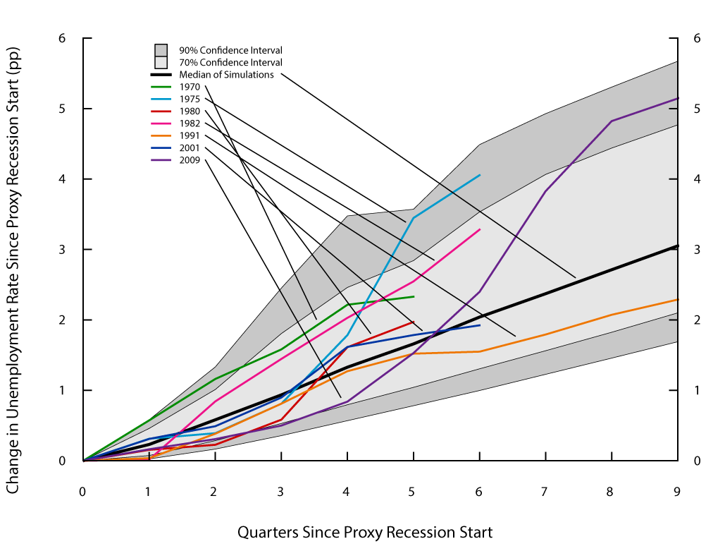
Another feature of the original simulation procedure that can be explored is its capability to generate unemployment rate trajectories during proxy recessions like those observed in the data. Figure 3 shows these trajectories for each of the seven historical proxy recessions considered and compares them with those produced by the model under the standard bootstrap. We plot the increase in the unemployment rate since the beginning of a proxy recession started. At any given quarter, the confidence intervals are composed of those simulated proxy recessions that last until that quarter or longer. Even though the median increase in the unemployment rate since a recession started (the black line) tends to overstate the increases in the data for short recessions, it understates the increase for long recessions--even the 90 percent confidence interval fails to cover the unemployment rate increases of the 1975, 1982, and 2009 recessions.
Thus, the standard bootstrap procedure delivers simulated recessions that are shallower, shorter, and less frequent than observed in history. Additionally, under the original procedure, the simulated recessions are unlikely to resemble the features of the unemployment rate observed during the Great Recession. Finally, the standard bootstrap has serious difficulties in generating increases in the unemployment rate as large as those observed during the worst recession episodes in history.
- An alternative stochastic simulation procedure
Why does the original stochastic simulation procedure fail to replicate key patterns of the data, even though the shocks are constructed as the residuals needed for the model to match the data over history?8 One possibility is that the assumption in the standard procedure about the independence of shocks during recession episodes is incorrect. In other words, shocks might be correlated across time. Drawing on that idea, we propose an improvement to the original procedure by clustering periods from non-recessions, conventional recessions, and the Great Recession in a probabilistic way.
To that end, we divide recession and non-recession periods according to the NBER denomination. We assume that the transition from non-recession to recession regimes is Markovian--i.e., it depends only on the current state and not on a longer history of data.9 Then, we calibrate a transition probability vector that is consistent with the average duration of non-recessions and the transition from non-recessions to recessions. In particular, the average duration of non-recessions during the 1970:Q1 to 2017:Q4 period is about 24 quarters,10 which implies that the probability of staying in a non-recession state is 0.958. Additionally, we have observed seven transitions from non-recessions to recessions, one of them to the Great Recession.11 Hence, the 0.042 probability of going to a recession from a non-recession regime is split according to these historical transition frequencies. The resulting transition probabilities are 0.036 to conventional recession regimes and 0.006 to the Great Recession regime.12
The simulation scheme is such that, once it is determined that the model switches from the non-recession regime to one of the two types of recessions, either one of the six conventional recessions is chosen randomly with equal probability or the Great Recession is selected. Once one of these recessions is chosen, the entire sequence of the shocks corresponding to that particular historical recession is run through the model. After all the shocks from that recession have run through, the procedure switches back to a non-recession regime and continues sampling residuals with replacement from that state with the probability indicated above.13 We refer to the alternative stochastic simulation procedure as the modified Markov-switching approach.14
Table 3 presents the results of the Markov-switching approach and compares them with the statistics from the data and with those obtained under the standard bootstrap simulation method that appeared in Table 2. The table shows that under this procedure, the model significantly improves its capacity to simulate deep recessions. Specifically, the median of simulated peak-to-trough increases in the unemployment rate is now 2.1 percentage points, a bit shy of the 2.2 percentage points estimated from the data. Furthermore, the 90th percentile increase in the unemployment rate of 4.3 percentage points is substantially higher than under the standard bootstrap method and is only about 3/4 percentage point below the maximum peak-to-trough increase observed in the data (not shown in the table). Regarding the duration of recessions, the proposed approach does not materially change the features observed under the standard bootstrap procedure. However, the median frequency of recession episodes (6) is closer to the data (7) than under the standard bootstrap (5), whereas its 90th percentile more than covers the frequency observed in history.
Table 3: Features of the modified Markov-switching simulation method
Statistics for peak-to-trough changes during proxy recessions
| Variable | Statistic | Data | Model (original) | Model (proposed) |
|---|---|---|---|---|
| Unemployment rate (pp) | median | 2.2 | 1.8 | 2.1 |
| 10th | 0.9 | 1.0 | ||
| 90th | 3.1 | 4.3 | ||
| Core PCE inflation rate (pp) | median | -0.3 | 0.0 | -0.2 |
| 10th | -1.3 | -1.6 | ||
| 90th | 1.4 | 1.6 | ||
| Federal funds rate (pp) | median | -4.8 | -1.1 | -1.2 |
| 10th | -3.1 | -3.9 | ||
| 90th | 0.4 | 0.8 |
Duration and frequency of proxy recessions
| Statistic | Data | Model (original) | Model (proposed) | |
|---|---|---|---|---|
| Length (quarters) | median | 6 | 5 | 5 |
| 10th | 4 | 4 | ||
| 90th | 9 | 9 | ||
| Frequency (episodes) | median | 7* | 5 | 6 |
| 10th | 3 | 4 | ||
| 90th | 7 | 8 |
* Corresponds to the recession episodes in the data. Return to table
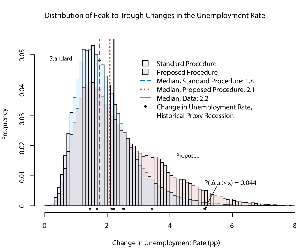
The ability of the model to generate extreme outcomes also improves with the proposed procedure. Consistent with the larger 90th percentile of peak-to-trough-increases of the unemployment rate described before, the proposed scheme delivers a frequency distribution that has significantly more mass around extreme events, as can be seen in Figure 4. In particular, among the set of recessions generated by the model, outcomes equal to or worse than those seen in the Great Recession happen more than 4 percent of the time.
Lastly, in terms of the model's trajectories, Figure 5 illustrates how, under the modified Markov-switching simulation method, the 90 percent confidence interval now includes all the trajectories observed in the data, although the median trajectory is only marginally higher than in the original procedure.
A shortcoming of both the original and the proposed procedure for running stochastic simulations in FRB/US is that the federal funds rate does not decline during recessions as sharply as in the data. Under both simulation approaches, the policy rate declines only a little more than 1 percentage point during recessions, compared with about 5 percentage points in the data, reflecting the inertial policy rule used in the simulations.
- The modified Markov-switching procedure around an SEP baseline
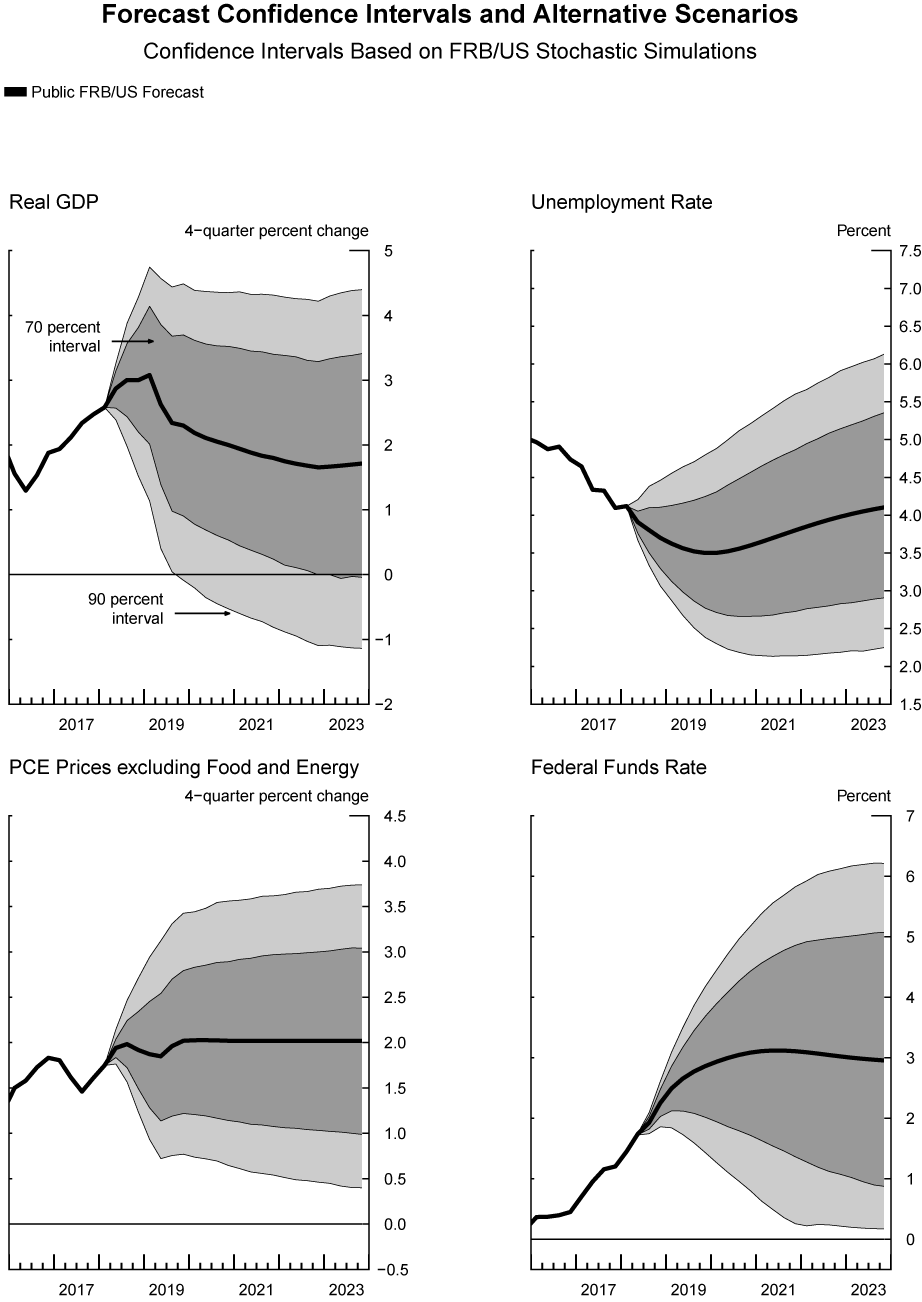
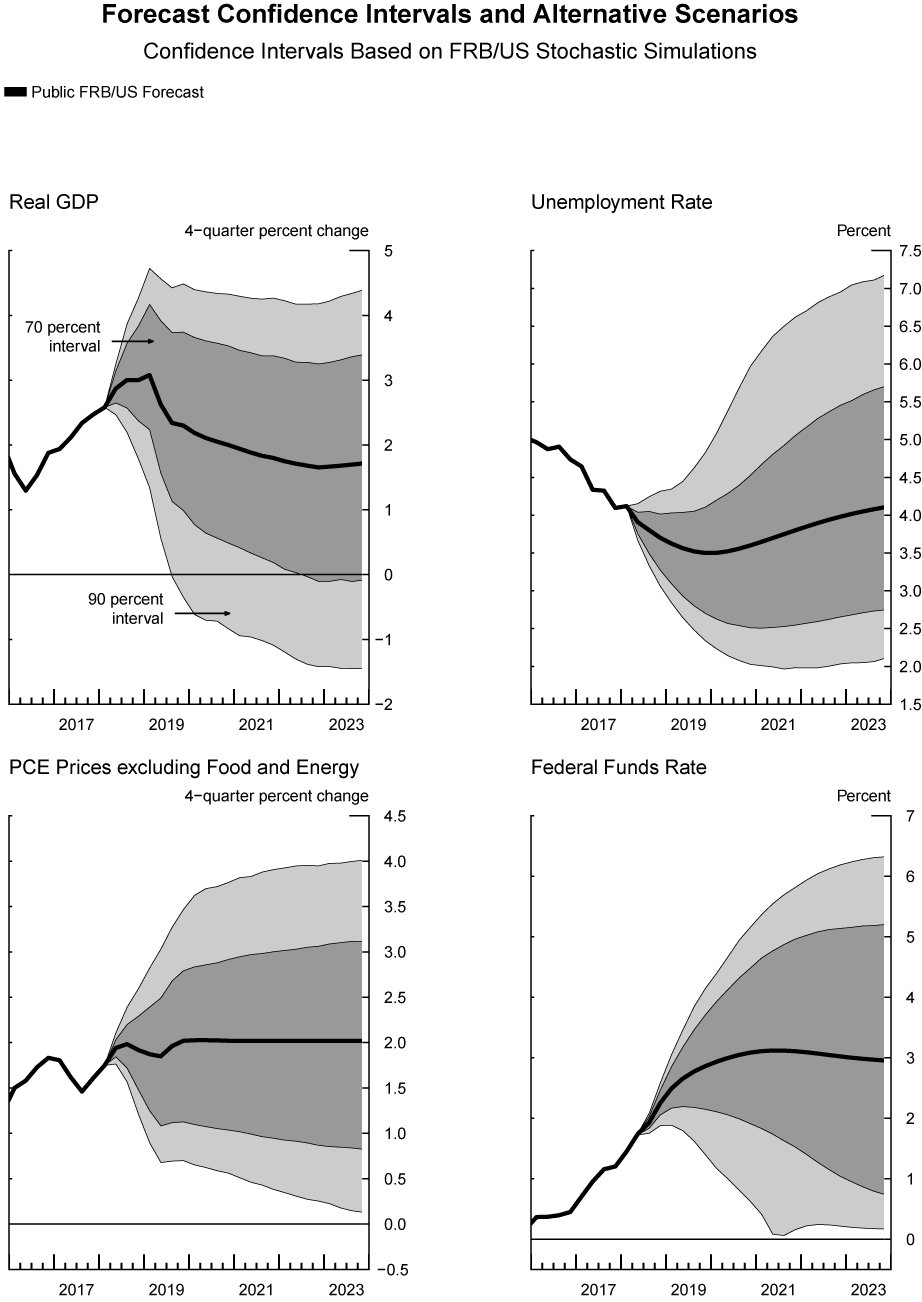
In this section, we apply the proposed modified Markov-switching simulation approach to produce confidence intervals around an SEP baseline. The stochastic simulations begin in 2018:Q2 and end in 2040:Q4. Because we are interested in outcomes in which the federal funds rate remains above the effective lower bound, we impose the ELB constraint, which was absent in the simulations shown in the previous sections. Figure 6 shows the long-run SEP baseline along with fan charts under the standard bootstrap methodology, whereas Figure 7 shows the long-run SEP baseline with fan charts under the modified Markov-switching procedure.
Figure 6 evidences that under the original methodology, the stochastic simulations generate mostly symmetric confidence intervals. For example, the 90 percent confidence interval for the unemployment rate forecast at the end of 2023 goes from roughly 2 1/4 percent to 6 1/4 percent, with the modal forecast just under 4 1/4 percent.
Under the new modified Markov-switching procedure in Figure 7, however, confidence intervals are asymmetric. In particular, the 90 percent confidence interval for the unemployment rate forecast at the end of 2023 goes from roughly 2 percent to 7 1/4 percent, about the same and about 1 percentage point higher, respectively, than under the standard bootstrap approach. However, the unemployment rate does not increase as rapidly in the short term under the modified Markov-switching procedure as in the standard bootstrap because we assume the current quarter is a non-recession period, which implies there is a higher probability of staying in that regime in the modified Markov switching than under the standard bootstrap approach that assumes independence among draws.
There are also differences in the confidence intervals for the other variables reported. For output growth, the stochastic simulations under the modified Markov-switching approach mirror the features of those of the unemployment rate. The simulations are more skewed to the downside in 2023, but are less likely to deliver low growth rates than the standard bootstrap in the short term.
For inflation, the two approaches deliver similar confidence intervals in terms of their symmetry, but the modified Markov-switching procedure includes more extreme inflation realizations in the confidence intervals. Finally, with respect to the federal funds rate, under the modified Markov-switching approach, the 90 percent confidence interval indicates that the ELB could bind in mid-2021, a feature that is absent in the standard procedure.
- Conclusions
This Fed Note introduced a novel procedure for generating stochastic simulations in FRB/US. The updated methodology relies on the fundamental assumption that adverse shocks in recessions tend to be correlated across time. By taking into account the serial correlation of residuals, this procedure is able to address some important concerns about the model's capacity to generate recessions of the same depth, duration, and frequency as observed in the data.
- References:
Board of Governors of the Federal Reserve System, 2012, "Tealbook A," Federal Open Market Committee (Transcripts and Other Historical Materials), www.federalreserve.gov/monetarypolicy/files/FOMC20121212tealbooka20121205.pdf [Accessed 30 Jul. 2018].
Board of Governors of the Federal Reserve System, 2018, "What is assumed about the cross and serial correlation of the shocks used in the stochastic simulation program?," The Fed - Technical Q&As. [online] Available at: https://www.federalreserve.gov/econres/us-technical-qas.htm#q13 [Accessed 30 Jul. 2018].
Board of Governors of the Federal Reserve System (US), Effective Federal Funds Rate [FEDFUNDS], retrieved from FRED, Federal Reserve Bank of St. Louis; https://fred.stlouisfed.org/series/FEDFUNDS, January 25, 2019
Kai Carstensen & Markus Heinrich & Magnus Reif & Maik H. Wolters, 2017. "Predicting Ordinary and Severe Recessions with a Three-State Markov-Switching Dynamic Factor Model. An Application to the German Business Cycle," CESifo Working Paper Series 6457, CESifo Group Munich. https://ideas.repec.org/p/ces/ceswps/_6457.html
Labor Force Statistics from the Current Population Survey https://data.bls.gov/timeseries/lns14000000.
James, D. Hamilton, "Regime Switching Models", Palgrave Dictionary of Economics, May 2005
U.S. Bureau of Labor Statistics, Civilian Unemployment Rate [UNRATE], retrieved from FRED, Federal Reserve Bank of St. Louis; https://fred.stlouisfed.org/series/UNRATE, January 25, 2019.
U.S. Bureau of Economic Analysis, Personal Consumption Expenditures Excluding Food and Energy (Chain-Type Price Index) [PCEPILFE], retrieved from FRED, Federal Reserve Bank of St. Louis; https://fred.stlouisfed.org/series/PCEPILFE, January 25, 2019.
1. The authors especially thank Zachary Price and Tilda Horvath for outstanding technology and research assistance that greatly contributed to the results presented here. Return to text
2. See FEDS Note "The FRB/US Model: A Tool for Macroeconomic Policy Analysis," April 2014, https://www.federalreserve.gov/econresdata/notes/feds-notes/2014/a-tool-for-macroeconomic-policy-analysis.html
3. The original approach does not draw residuals from the equation for the monetary policy rule. The rationale for this is that the stochastic simulations were purely conditional on an interest rate rule. This feature remains the same in the proposed procedure described later in the paper. Also, note that the role of the SEP baseline in this case is merely a descriptive one, because in any linear model solved in deviations, a specific baseline will solely introduce level differentials to the model's solution values. Return to text
4. As they appear, for instance, in the Risks & Uncertainty section of Tealbook A (see Tealbook A from December 2012 pp. 83-95 in https://www.federalreserve.gov/monetarypolicy/files/FOMC20121212tealbooka20121205.pdf). Return to text
5. Although the simulations are conducted using the SEP baseline roughly at steady-state, the joint distribution of initial conditions at that time and shocks under the proposed Markov-switching procedure described later may need some time to reach the stationary distribution, which is why the initial 60 quarters were dropped. Initial conditions are innocuous under the standard bootstrap method. Return to text
6. Our choice not to impose the effective lower bound can be seen as, in part, reflecting the idea that monetary policy has other tools available when the short-term interest rate becomes constrained, but these other tools are much harder to model. In turn, addressing a related concern–the distribution of episodes associated with a binding ELB on the nominal federal funds rate–requires a realistic distribution of adverse events. However, with only one observed episode at the ELB, assessments of the model-implied distribution are less straightforward and would require specific assumptions about, for example, the conduct of monetary policy under those circumstances. These assumptions would be hard to test with the limited data at hand. We have also added a cyclically adjusted federal government target surplus rule with the aim of improving the cyclical features of some fiscal variables of the model. It turns out that this adjustment improves the dynamic properties of the model when the ELB of interest rates is imposed in long simulations. In particular, the possibility of absorbing states in which the unemployment rate increases without bound as the simulation horizon increases is almost eliminated. Return to text
7. Another option would be to use the conventional criterion of two consecutive quarters of declining real GDP. However, this criterion does not identify periods that coincide closely with the NBER recession periods. Return to text
8. Recall that the procedure to generate the stochastic simulations does not use the residual of every equation of the model. Most notably, it does not use shocks to the monetary policy rule. In addition, some of the excluded residuals belong to trend equations that can have problematic long-run properties. Return to text
9. This assumption is consistent with the view that expansions do not die of old age; that is, the probability of exiting from an expansion is independent of its duration. Return to text
10. For calculating the transition probabilities, we assume the current non-recession period that began in 2009:Q3 ended in 2017:Q4. Also, we do not take into account the four non-recession quarters in place before 1970:Q1. Return to text
11. In the seven transitions, we account for the transition to the first recession in the sample, which started in 1970:Q1. Return to text
12. The transition probability from the non-recession regime to the Great Recession, which is equal to 0.006, is a key parameter in the analysis, but unfortunately one that is highly uncertain. One could argue that the true probability is much lower given that one would have to go all the way back to 1929 to see an event similar to the Great Recession; alternatively, one might worry that the true probability is higher because the risk of financial instability emerging is high in a world of persistently low interest rates. As will be shown, this parameter value is enough to help reproduce satisfactorily the historical events in the sample used, which is our criterion to keep it. Return to text
13. We verified that this proposed procedure does not generate biased trajectories. At the end of 200 quarters and averaging over simulations, real GDP is 0.04 percentage point higher than in the long-run SEP baseline, while the unemployment rate is 0.1 basis point higher. Return to text
14. The Markov switching in this methodology is modified in the sense that the transitions from recession to non-recession states is deterministic and not stochastic like in a traditional Markov chain. Return to text
González-Astudillo, Manuel, and Diego Vilán (2019). "A New Procedure for Generating the Stochastic Simulations in FRB/US," FEDS Notes. Washington: Board of Governors of the Federal Reserve System, March 7, 2019, https://doi.org/10.17016/2380-7172.2314.
Disclaimer: FEDS Notes are articles in which Board staff offer their own views and present analysis on a range of topics in economics and finance. These articles are shorter and less technically oriented than FEDS Working Papers and IFDP papers.