FEDS Notes
May 06, 2019
Predicting Future Recessions
Summary
This note introduces a general method to derive recession probabilities from forecasts using real-time data in parsimoniously specified logistic regressions. I apply two specifications of the general method that produces an implied recession probability to forecasts contained in releases of the Survey of Professional Forecasters (SPF). Using yearly forecasts from the 2018:Q3 SPF, the probability of a recession peaks between 30 percent in 2020 and 40 percent in 2021. Using quarterly forecasts, the probability of a recession within four quarters is monotonically increasing during the forecast, hitting a high between 35 and 40 percent in 2019:Q3.
Introduction
Recessions are notoriously difficult to predict. The difficulty comes from a lack of recessions--there have only been seven since 1965, each lasting around a year on average--and a related lack of understanding of what causes them. Given these limitations, it is not surprising that forecasts of economic variables rarely explicitly include a recession. However, forecasts may include conditions, outside of output and unemployment, which have presaged previous recessions and thus may be analyzed to produce an implied recession probability.
The general method to produce an implied recession probability from a forecast has the following steps. First, choose a subset of variables included in the forecast, excluding output and unemployment, which are correlated with expansions and recessions. Second, estimate a logit using real-time historical data for those variables and a dependent variable that is an indicator of an incoming recession. Finally, apply the logit to the data provided by the forecast to generate the probability that a recession occurs during the forecast period.1
Source: Author's calculations based on forecasts from 2018q3 SPF.
Source: Author's calculations based on forecasts from 2018q3 SPF.
In this note, I analyze the forecasts provided by the SPF. Each release of the SPF contains quarterly forecasts for up to a year and yearly forecasts for up to three years beyond the SPF's publication date for a large number of variables. To illustrate the power and robustness of the general method, I design two different logits, using unique independent variables constructed from the SPF, and estimate them at the two different frequencies using real-time data.
The first logit uses forecasts of the yield curve to predict recessions. I use the 10-year Treasury bond minus the 3-month Treasury bill yield curve, which has a well-known history of successfully predicting recessions. The second logit uses two variables whose analogs can be found in the SPF: the real federal funds gap, which is the difference between the real federal funds rate and the real equilibrium interest rate r*, and the unemployment gap, which is the difference between the unemployment rate and the equilibrium unemployment rate u*--also known as non-accelerating inflation rate of unemployment (NAIRU).
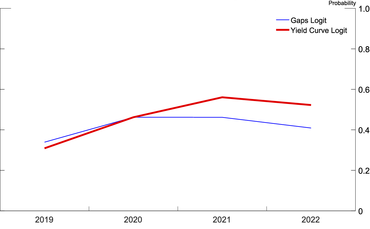
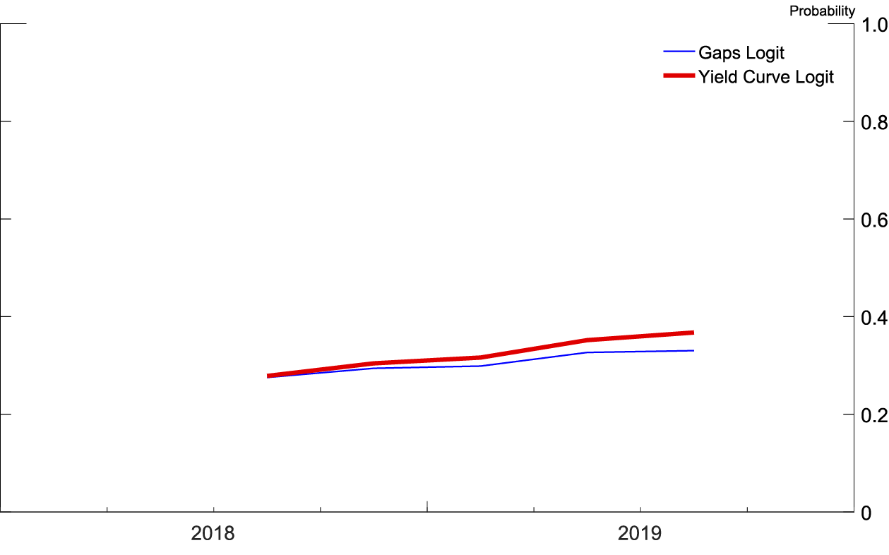
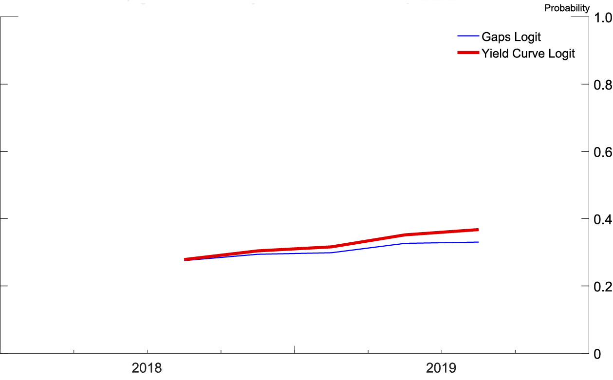
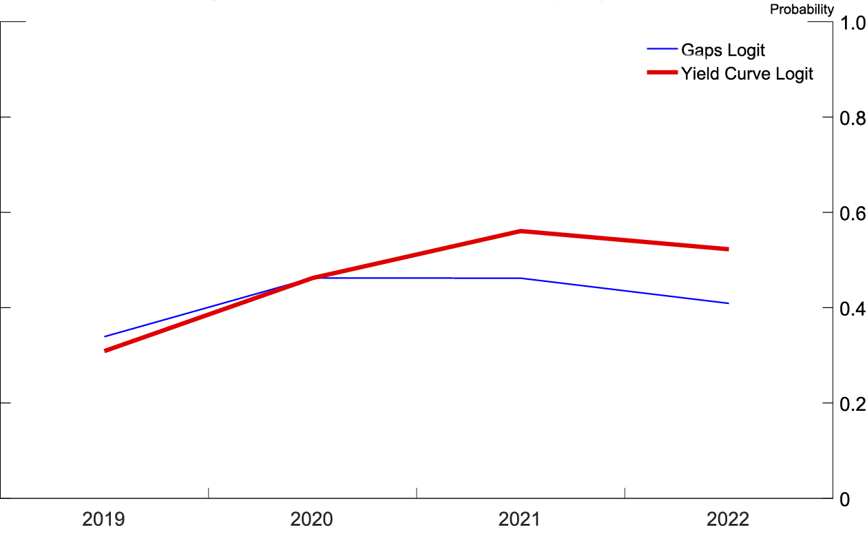
To preview results, both logits, at both frequencies, show that the probability of a recession has been steadily increasing since 2014. As shown in figure 1, at a yearly frequency, the recession probability model based on the yield curve peaks at a 40 percent chance of a recession occurring in 2021, while the recession probability model based on the unemployment and real federal funds gaps peaks at a 30 percent chance of a recession occurring in 2020. As shown in figure 2, at a quarterly frequency, both recession probability models are monotonically increasing over the forecast horizon, ending the forecast horizon showing between a 35 and a 40 percent chance of a recession within four quarters of 2019:Q3.
Methodology
In this section, I describe the construction of the logits, the real-time historical data on which the independent variables are estimated, the forecasts used, and the recession indicating dependent variables. For each SPF survey, there is a unique logit estimated using real-time data. I gather real-time data in order to align the data used to estimate the logit with the information sets of the SPF respondents at the time each SPF was published. For simplicity, I refer to the logits as singular. I use median SPF forecasts. Unless otherwise noted, data is from ALFRED, the archival economic database.
The first logit predicts recessions using the spread between the 10‑year Treasury bond and 3‑month Treasury bill. Constructing the real-time historical series on which the logit is estimated is simple because Treasury yields are known in real time and not updated. The SPF directly includes forecasts of both the 3-month Treasury bill (the variable TBILL in the SPF) and the 10-year Treasury bond (TBOND).2
The second logit predicts recessions using the real federal funds gap and the unemployment gap. I first construct the real-time historical series for the two gaps. Second, I calculate the gaps themselves from the SPF forecasts.
In constructing the unemployment gap, while the unemployment rate is known (with some lag), the equilibrium unemployment rate u* (also known as the NAIRU) is never observed. As an estimate of the equilibrium rate, I use the Congressional Budget Office's (CBO) estimate of the long-term natural rate of unemployment. The difference between the unemployment rate and the estimated long-term natural rate of unemployment is the unemployment gap.
To construct the real federal funds gap, a similar issue arises: While the federal funds rate is known, the equilibrium federal funds rate r* is never observed.3 As an estimate of the longer-run rate, I use the real-time estimates of r* generated by the Laubach and Williams (2003) model that are provided by the New York Federal Reserve.4 Because r* is a real interest rate while the federal funds rate is nominal, I deflate each year's federal funds rate by that year's personal consumption expenditures (PCE) price index growth to produce a historical real federal funds rate series.5 The difference between the real federal funds rate and the estimated r* is the real federal funds rate gap.
Construction of the historical gaps comes with caveats. Estimates of r* and u* are imprecise, subject to revision, and key to the calculation of both gaps. Using real-time data from the most commonly cited publicly available estimates addresses this concern as much as currently possible.
The SPF does not directly include the unemployment gap and real federal funds gap. I calculate the unemployment gap from each SPF using the difference between the unemployment rate (UNEMP) and the last reported forecast of u* (UBAR).6 To calculate the real federal funds gap, I use the difference between the 3-month Treasury bill (TBILL) and the annual average rate on 3-month Treasury bills over the next 10 years (BILL10), deflated by their respective PCE price index growth forecasts (PCE, PCE10).7 Thus the real federal funds gap incorporates a measure of the PCE gap, which is the difference between the forecast for PCE price index growth and the Federal Reserve's target PCE price index growth.
While the 3-month Treasury bill and the average 3-month Treasury bill over the next 10 years are not identical to the federal funds rate and equilibrium federal funds rate, they are closely related. The 3-month Treasury bill tracks the federal funds rate tightly. The average 3-month Treasury bill over the next 10 years should, for the most part, average over years when the federal funds rate, and thus the 3-month Treasury bill, is at its equilibrium value. Taking the difference between the 3-month Treasury bill and average 3-month Treasury bill over the next 10 years will eliminate any premium specific to the 3-month Treasury bill.
For quarterly regressions, each logit's dependent variable is an indicator that at least one of the next four quarters is judged by the National Bureau of Economic Research (NBER) to be a recession. In order to make the data real time, I assume, for simplicity, that the NBER recession dating occurs concurrent with the period judged to be a recession.8 For example, the logit estimated using real-time data as of 2001:Q2 has a dependent variable that indicates the economy was in recession in 2001:Q2, although the NBER would not officially make its recession declaration until 2001:Q3. For yearly regressions, I count a year as a recession year if at least one month of that year is contained in an NBER-dated recession.
Results
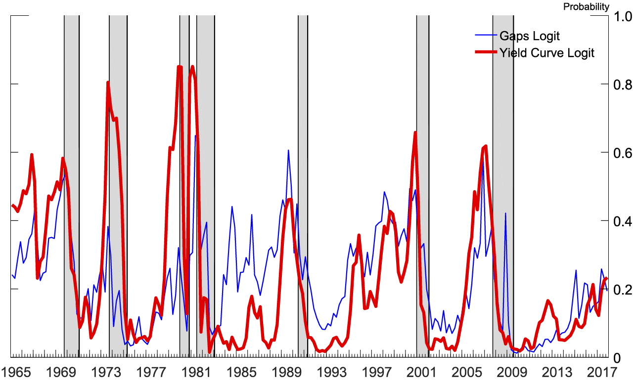
Note: The gray shaded bars indicate quarters that are in a business recession as defined by the National Bureau of Economic Research.
Source: Author's calculations based on forecasts from 2018q3 SPF.
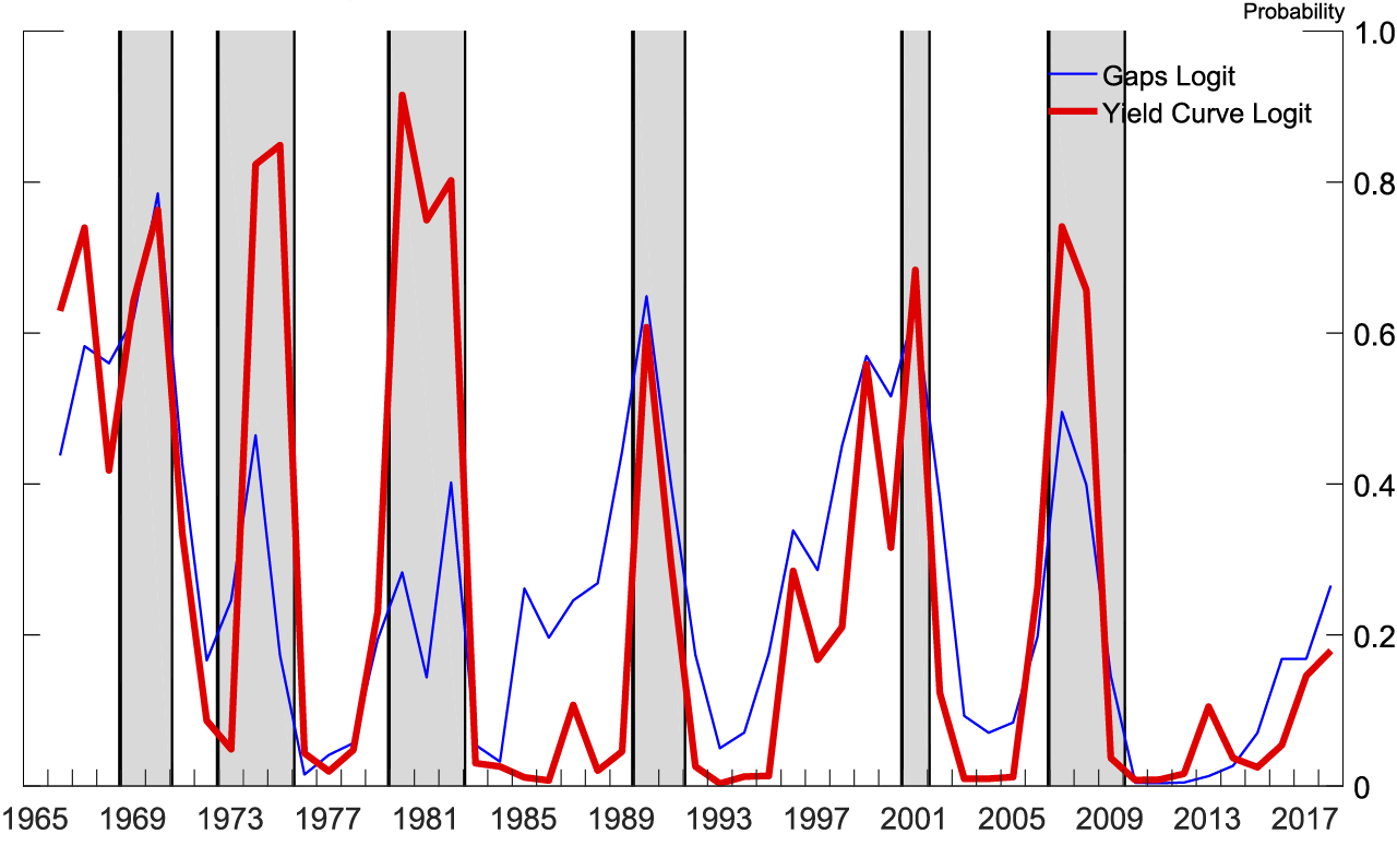
Note: The gray shaded bars indicate years with a period of business recession as defined by the National Bureau of Economic Research.
Source: Author's calculations based on forecasts from 2018q3 SPF.
Figure 3 shows how the two logits estimated using real-time data for the 2018:Q3 SPF fit over quarterly history. All independent variables are statistically significant at the 1 percent level in their respective logits. Figure 4 shows how the two logits estimated using real-time data for the 2018:Q3 SPF fit over yearly history. The yield curve is significant at the 1 percent level in its logit. The unemployment gap is significant at the 1 percent level and the real federal funds gap at the 10 percent level in their logit. Independent variables in logits estimated for earlier SPF surveys have similar significance.
Source: Author's calculations based on forecasts from 2018q3 SPF.
Source: Author's calculations based on forecasts from 2018q3 SPF.
Figures 5 and 6 (similar to figures 1 and 2) show the probability of recession derived from the 2018:Q3 SPF using both logits at both frequencies. In figure 5, at a quarterly frequency, both recession probability models are monotonically increasing over the forecast horizon, ending the forecast horizon showing between a 35 and a 40 percent chance of a recession within four quarters of 2019:Q3. In figure 6, at a yearly frequency, the recession probability derived from the yield curve based logit peaks at a 40 percent chance of a recession occurring in 2021, while the recession probability derived from the logit based on the unemployment and real federal funds rate gaps peaks at a 30 percent chance of a recession occurring in 2020.
The increasing probability of a recession in the yield curve logit comes from the well-known result that yield curve inversions presage recessions. The forecasts include a flatter yield curve, making an inversion more likely, thus the probability of a recession is higher. For the logit based on the unemployment gap and real federal funds rate gap, the coefficients on the gap variables in the logit show that the further the unemployment rate is below its equilibrium value and the higher the real federal funds rate is above its equilibrium value, the higher the probability of a recession. In other words, recessions are most likely when the economy is "running hot" and the Federal Reserve has raised the real federal funds rate above its longer-run value in order to cool off the economy. The logit is responding to the Federal Reserve's historical difficulty in engineering soft landings to expansions, and, by definition, all expansions end with a recession.
Note: The gray shaded bars indicate quarters that are in a business recession as defined by the National Bureau of Economic Research.
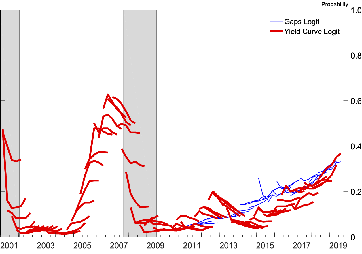
Source: Author's calculations based on forecasts from all SPFs since 2001q1 SPF.
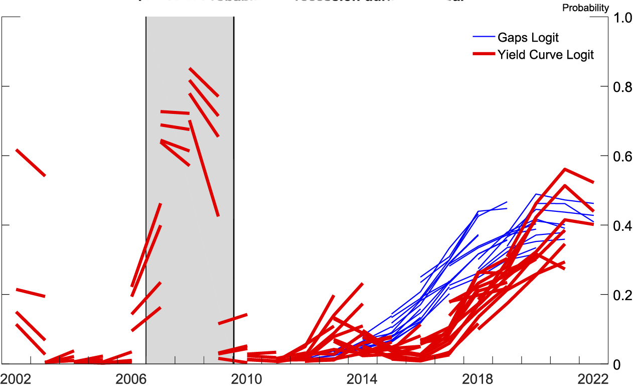
Note: The gray shaded bars indicate years with a period of business recession as defined by the National Bureau of Economic Research.
Source: Author's calculations based on forecasts from all SPFs since 2001q1 SPF.
Figures 7 and 8 display the recession probabilities from all SPF forecasts since the 2001:Q1 SPF. Each line is the implied recession probability from a single SPF over that SPF's forecast horizon, generated by a logit estimated with real-time data available at the time of that SPF's publication.9 As can be seen, the yield curve logit was good at forecasting the Great Recession. In both logits, after 2014 the probability of a recession has been rising nearly monotonically in the forecasts as the yield curve flattens and the soft landing nears.
Conclusion
Comparing forecasts with their historical antecedents can produce a measure of the probability of a recession, even when no recession is explicitly forecast. The simple method of using a parsimonious logit estimated on historical data applied to a forecast produces a good measure of the probability of a recession. Choosing which variables from the forecast to include in the logit and how to build the historical analogs of those variables takes consideration and understanding of economic relationships.
References
Bauer, Michael D., and Thomas M. Mertens (2018). "Economic Forecasts with the Yield Curve," FRBSF Economic Letter 2018-07 (San Francisco: Federal Reserve Bank of San Francisco, March 5), https://www.frbsf.org/economic-research/publications/economic-letter/2018/march/economic-forecasts-with-yield-curve.
Laubach, Thomas, and John C. Williams (2003). "Measuring the Natural Rate of Interest," Review of Economics and Statistics, vol. 85 (November), pp. 1063–70.
1. While this method has previously been applied to historical data, usually using the yield curve as an independent variable as in Bauer and Mertens (2018), it is not used to analyze forecasts themselves. Return to text
2. The SPF includes a different variable, SPR_TBOND_TBILL that directly calculates the spread. There is little difference in forecasts using the two different constructions. Return to text
3. While data and estimates exist for the federal funds rate target from 1982 to the present, the federal funds rate target is unknown from 1965 to 1981. I use the average of the effective federal funds rate for those years. Return to text
4. Federal Reserve Bank of New York, Measuring the Natural Rate of Interest, https://www.newyorkfed.org/research/policy/rstar/overview. Return to text
5. Using real rates is necessary because the Federal Reserve did not have an explicit inflation target over history that could be used to inflate the r* estimates. In order to use nominal quantities, you would need a time-varying estimate of the Federal Reserve's inflation target. Return to text
6. The SPF provides an estimate of the natural rate of unemployment only in third-quarter surveys. Return to text
7. The SPF explicitly provides forecasts for four years of all variables except PCE price index growth, where it provides three years. The forecast for the fourth year of PCE price index growth is imputed using the three years of forecast PCE price index growth provided and the forecast for average PCE price index growth over the next five years (PCE5YR). Return to text
8. Using the true dates of the NBER recession declaration makes little difference (and would involve a judgement of when individuals in the economy understand they are in a recession). For more information, see https://www.nber.org/cycles/recessions_faq.html. Return to text
9. Forecasts using the unemployment gap and real federal funds gap logit start in 2012 due to real-time data availability limitations of the CBO's estimate of u*. Yearly forecasts for yield curve variables were for 1 year past the release date until the 2009:Q3 SPF. Return to text
Miller, David S. (2019). "Predicting Future Recessions," FEDS Notes. Washington: Board of Governors of the Federal Reserve System, May 6, 2019, https://doi.org/10.17016/2380-7172.2338.
Disclaimer: FEDS Notes are articles in which Board staff offer their own views and present analysis on a range of topics in economics and finance. These articles are shorter and less technically oriented than FEDS Working Papers and IFDP papers.