FEDS Notes
February 25, 2021
Quantifying the COVID-19 effects on core PCE price inflation
Matteo Luciani
The 12-month change in core PCE price inflation was 1.5 percent in December. Why was core inflation so low in 2020? How much of this weakness can be attributed to the COVID pandemic? And what does this mean for inflation going forward?
In this note, I answer these questions by using an entirely data-driven model—in other words, I do not make any "structural" economic assumptions or ad hoc judgments about what factors are affecting prices—to estimate the effects of COVID on core PCE prices.
Methodology
To estimate the effects of COVID on core PCE price inflation, I use a Dynamic Factor model estimated on a large dataset of disaggregated prices. Here I provide an intuitive description of the model, while in the Technical Appendix, I provide a more technical description.
The model that I use decomposes core inflation ($$\pi^c_t$$) into
- a common component ($$\chi^c_t$$), also called common core inflation (Luciani 2020), that captures changes in prices that are common to many or all prices but that excludes the effect of COVID on the comovement of prices;
- a COVID component that captures COVID-induced comovement ($${C19}^C_t$$);
- and an idiosyncratic component ($$\xi^c_t$$), which captures relative price movements that reflect sector-specific developments and measurement error:
$$ \pi^c_t = \chi^c_t + {C19}^C_t + \xi^c_t . $$
The comovement among disaggregated PCE prices captured by the common component has been quite stable over time. However, as shown in Figure 4 in the Technical Appendix, this stability broke down this year because COVID introduced additional/unusual comovement among prices.
Now, what does it mean that COVID introduced additional/unusual comovement among disaggregated PCE prices? It means that in March and April 2020, most disaggregated prices declined in response to the disruption induced by the lockdown. In particular, many COVID-sensitive prices (e.g., airfares and accommodation prices) whose movements are normally idiosyncratic moved together with several other prices. Therefore, the comovement during COVID is unusual because it incorporates much more of the movement of these normally highly idiosyncratic categories.
This new pattern of comovement offers the possibility to identify the COVID component. Specifically, I estimate the COVID component by comparing the pattern of comovement during COVID ($$\hat{\chi}^c_t$$) with the stable pattern of comovement before COVID ($$\tilde{\chi}^c_t$$): $$\widehat{C19}^C_t = \hat{\chi}^c_t - \tilde{\chi}^c_t$$, if $$ t \ge \text{2020: M3}$$, otherwise $$\widehat{C19}^C_t = 0$$.1
Empirical analysis
I estimate the model on a dataset of 146 monthly PCE price indexes from January 1995 to December 2020. The dataset used to estimate the model represents a particular disaggregation of PCE prices in which each disaggregated price index is constructed from a distinct data source (see Luciani, 2020, for details).
Figure 1 shows the decomposition of monthly core PCE price inflation, where the red line is common core inflation, the orange line is the COVID component, and the blue line gives the idiosyncratic component. By construction, these three components sum to overall core PCE inflation, which is shown in the plot as a black line.
Monthly percent change
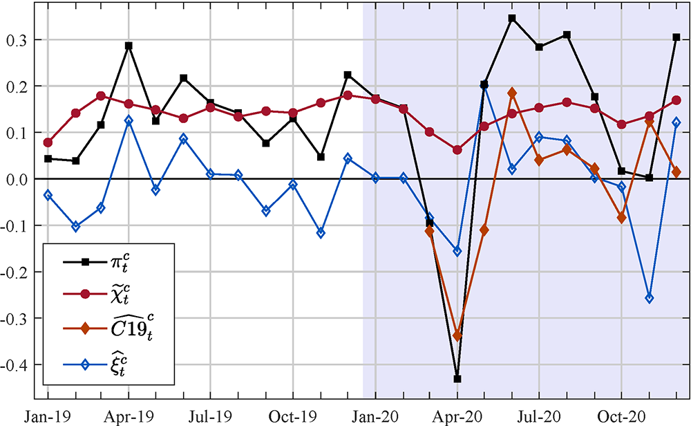
Notes: the red line is the common core inflation, the orange line is the COVID component, while the blue line gives the idiosyncratic component. By construction, these three components sum to overall core PCE inflation (the black line).
According to the model estimate, COVID lowered core PCE price inflation in March, April, and May by about ½ percentage point, when the COVID component was primarily driven by the price index for financial services, apparel, non-profit institutions serving households, used cars, accommodation, and airfares (Table 1, second-to-fourth columns). In contrast, COVID boosted core PCE price inflation in June by about 0.2 percentage point and in November by about 0.1 percentage point, when the COVID component was primarily driven by the price index for financial services, apparel, non-profit institutions serving households, used cars, accommodation, and airfares (Table 1, fifth and sixth columns).
Table 1: Contribution of selected prices to the estimated COVID component* †
| Mar. | Apr. | May | Jun. | Nov. | Mar.-Dec. | |
|---|---|---|---|---|---|---|
| Net Purchases of Used Motor Vehicles | -1.7 | -4 | 1.5 | 3.2 | 2.8 | 2.7 |
| Furniture | -0.5 | -1.3 | 0.4 | 0.7 | 0.7 | -0.2 |
| Apparel** | -2.3 | -5.5 | -2.8 | 4.1 | 1.4 | 0 |
| Housing‡ | 0.3 | -0.2 | -0.3 | -1.7 | -0.1 | -5.1 |
| Physician Services | -0.1 | -0.4 | 0.2 | -0.2 | 0.3 | -1.1 |
| Paramedical Services | 0 | -0.2 | 0.1 | -0.3 | 0.1 | -1.2 |
| Hospitals | -0.1 | -0.6 | 1.1 | -0.5 | 0.8 | -2.1 |
| Motor Vehicle Rental | -0.5 | -1 | -0.1 | 0.5 | 0.4 | -0.3 |
| Air Transportation | -1.5 | -1.5 | 0.3 | 0.7 | 1.7 | -1.4 |
| Hotels and Motels | -1.2 | -1.8 | -0.2 | 0.7 | 0.6 | -1.6 |
| Pension Funds | -0.5 | -2 | -0.1 | 1.1 | 0.7 | -0.6 |
| Financial Service Charges, Fees & Commissions | -1.8 | -9.5 | -6.4 | 7.8 | 1.4 | -1.4 |
| Life Insurance | 0.1 | 1.4 | -1.1 | -1.4 | -1.1 | -0.8 |
| Net Health Insurance | 0.1 | -0.2 | -0.1 | -0.3 | 0.1 | -1.3 |
| Communication | -0.1 | -0.4 | 0.1 | -0.2 | 0.2 | -1 |
| Higher Education | 0.1 | 0 | -0.2 | -0.4 | -0.1 | -1.3 |
| Nonprofit Institutions Serving Households | -0.8 | -4.7 | -4.9 | 2.9 | 0.2 | -3.9 |
* This table reports $$\widehat{C19}^c_{it} = \hat{\chi}^c_{it} - \tilde{\chi}^c_{it}$$, where the unit of measure of $$\hat{C}^c_{i,19}$$ is basis points. The prices reported in the table satisfy one of these criteria: $$\widehat{C19}^c_{it} \le -1$$ for $$t =$$ March, April, or May 2020, $$\widehat{C19}^c_{it} \ge 1$$ for $$t =$$ June or November 2020, or $$\sum_{t=t_0}^T \widehat{C19}^c_{it} \le -1 $$ where $$t_0 =$$ March 2020 and $$T =$$ December 2020.
† Highlighted cells are referred to in the text.
** Apparel is the sum of "Men's & Boys' Clothing," "Women's & Girls' Clothing," and "Shoes & Other Footwear."
‡ Housing is the sum of "Rent of primary residence" and "Imputed Rental of Owner-Occupied Nonfarm Housing."
Figure 2 shows the decomposition of the 12-month change in core PCE price inflation. Here, the red line tells us what core inflation would have been had there been no COVID shock and no idiosyncratic price shocks over the past 12 months, while the difference between the red and the green line gives us the contribution of COVID to 12-month percent change in core PCE price inflation. As can be seen, the model estimates that COVID shaved cumulatively about 0.2 percentage point off common core inflation through December, primarily driven by the price index for Housing, Non-Profit Institutions, and hospitals (Table 1, last column).
To conclude, what is the implication of these results for inflation going forward? To answer this question it is necessary to understand what the statistical properties of $$\widehat{C19}^c_t$$ are. Now, the difference ($$\hat{\chi}^c_t - \tilde{\chi}^c_t$$) is by construction a zero-mean stationary variable, and so over the whole sample, its mean is equal to zero by construction.2 Therefore, $$\widehat{C19}^c_t$$ is a stationary variable; however, for $$t \ge \text{2020: M3}$$, its sample mean is not necessarily equal to zero (right now, it has a mean of about 2 basis points), but as more observations come in, it will converge toward zero. Hence, provided that the effects of the COVID pandemic on the economy will fade away this year or next, it is reasonable to expect that, following the very low readings between March and May, $$\widehat{C19}^c_t$$ will rebound in the near future.
12-month percent change
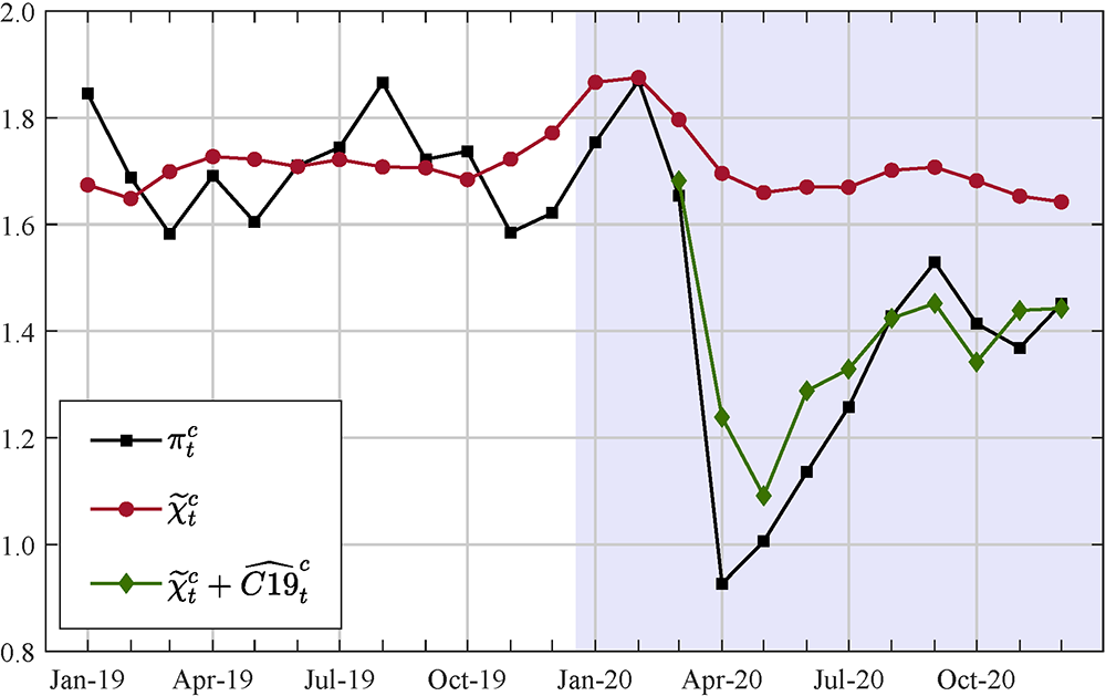
Notes: the red line is common core inflation, the green line is the sum of the common core inflation and the COVID component, $$\tilde{\chi}^c_t + \widehat{C19}^c_t$$, and the black line is core PCE price inflation.
Conclusions
In this note, I first document that COVID induced an additional and unusual comovement among PCE prices, and then I show how by isolating this extra-comovement, I am able to provide a novel estimate of the effect of COVID on prices. I find that the COVID-induced additional comovement had an important negative effect on prices in 2020. However, because this extra comovement is simply a result of the COVID shock, and to the extent that the effects of COVID on activity disappear sometimes this or next year, the model would expect inflation in COVID-affected prices to boost core inflation in the near future.
References
Barigozzi, M, and Luciani, M. (2020). "Quasi Maximum Likelihood Estimation and Inference of Large Approximate Dynamic Factor Models via the EM algorithm," arXiv:1910.03821v2.
Luciani, M. (2020). "Common and idiosyncratic inflation," Finance and Economics Discussion Series 2020-024. Washington: Board of Governors of the Federal Reserve System.
Technical Appendix
Model Estimation
The model is estimated in three steps: in the first step, I decompose the rate of change for each individual price index into a common and an idiosyncratic component by estimating a dynamic factor model. In the second step, I aggregate the common components using weights of the series in the overall core PCE price index. In the third step, I compute the COVID component by exploiting a break in the comovement in PCE prices that occurred with COVID.
Step 1: Let $$\pi_{it}$$ be the month-on-month inflation rate for item $$i$$ at time $$t$$, then the dynamic factor model used in this note is
$$(1) \ \ \ \ \pi_{it} = \chi_{it} + \xi_{it} $$
$$(2) \ \ \ \ \chi_{it} = \lambda_{i0}f_t + \lambda_{i1}f_{t-1} + \lambda_{i2}f_{t-2} $$
$$(3) \ \ \ \ f_t = \phi_1f_{t-1} + \phi_2f_{t-2} + \phi_3f_{t-3} + u_t $$
where $$\chi_{it}$$ is the common component, $$\xi_{it}$$ is the idiosyncratic component, $$f_t$$ is the common factor, and $$\lambda_{is}$$ is the factor loading of price $$i$$ at lag $$s$$ — for a more formal and exhaustive treatment of the model, I refer the reader to Luciani (2020).
The model is estimated by Quasi-Maximum Likelihood (QML), implemented through the Expectation-Maximization (EM) algorithm (for a formal treatment of the EM algorithm, I refer the reader to Barigozzi and Luciani, 2020). Intuitively, at each iteration, given an estimate of the parameters, the factors are estimated by running the Kalman smoother (E-step). Then, given the estimate of the factors, the parameters are estimated equation-by-equation by running OLS, where the OLS formulas are modified to account for the estimation error in the estimated factors (M-step). This process is repeated until convergence, and after convergence of the EM algorithm, the Kalman Smoother is run for one last time.
Step 2: Let $$\hat{\chi}_{it}$$ be the estimated common component for item i, then common core inflation is estimated as
$$(4) \ \ \ \ \hat{\chi}^c_t = \sum_{i \in core} w_{it}\hat{\chi}_{it} = \sum_{i \in core} w_{it}(\hat{\lambda}_{i0}\hat{f}_t+\hat{\lambda}_{i1}\hat{f}_{t-1}+ \hat{\lambda}_{i2}\hat{f}_{t-2}) $$
where $$w_{it}$$ are the "approximate" PCE weights.3
Step 3: Let $$\hat{\chi}^c_t$$ be the estimate of common core inflation obtained by estimating the model on the whole sample. And let $$\tilde{\chi}^c_t$$ be the estimate of common core inflation obtained by estimating the parameters of the model—i.e., the $$\lambda$$s, the $$\phi$$s, and the variances of $$\xi_{it}$$ and $$u_t$$—on the sample ending in February 2020, while the factor is estimated over the full sample.4 Then I can define the effect of COVID on core PCE prices as
$$(5) \ \ \ \ \widehat{C19}^c_t = \Bigg\{ \begin{array}{ll} 0 & \text{ if }t \le \text{2020: M2} \\ \hat{\chi}^c_t-\tilde{\chi}^c_t & \text{ if }t \ge \text{2020: M3}\\ \end{array}, $$
and the idiosyncratic component is estimated as
$$\ \ \ \ \ \ \ \ \ \hat{\xi}^c_t = \Bigg\{ \begin{array}{ll} \pi^c_t - \hat{\chi}^c_t & \text{ if }t \le \text{2020: M2} \\ \pi^c_t-\tilde{\chi}^c_t & \text{ if }t \ge \text{2020: M3}\\ \end{array}. $$
The definition of the COVID component given in (5) implicitly assumes that $$\hat{\chi}^c_t$$ contains both the standard comovement as well as the additional/unusual comovement induced by COVID. Figure 3 shows both the monthly percent change and the 12-month change of $$\hat{\chi}^c_t$$ and $$\tilde{\chi}^c_t$$. The left chart in Figure 3 shows that pre-Covid-19 $$\hat{\chi}^c_t$$ captures approximately the same signal as $$\tilde{\chi}^c_t$$, but with larger fluctuations. Likewise, by looking at the right chart in Figure 3, it is clear that $$\hat{\chi}^c_t$$ captures a larger fraction of the decline in core PCE price inflation during the pandemic than $$\tilde{\chi}^c_t$$. In summary, the evidence provided in Figure 3 shows that $$\hat{\chi}^c_t$$ is capturing the same signal as $$\tilde{\chi}^c_t$$ plus something else, thus supporting the definition of the Covid-19 effect given in (5).
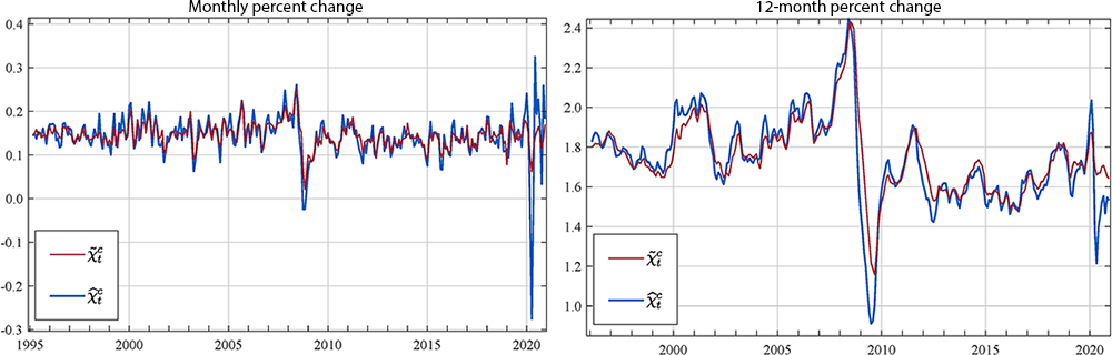
Notes: $$\hat{\chi}^c_t$$ is the estimate of common core inflation that contains both the standard comovement as well as the additional/unusual comovement induced by COVID, whereas $$\tilde{\chi}^c_t$$ does not contain COVID.
COVID induced a structural break
My identification of the COVID component relies on the fact that COVID induced a structural break in 2020. Because the estimated factor loadings, the $$\lambda$$s in equation (2), capture the comovement among prices, by comparing the $$\lambda$$s estimated on different samples, I can see how the comovement among prices has evolved over time.5
Figure 4 reports the cross-correlation between the factor loadings estimated on the sample ending at time $$t$$ and the those estimated on the sample ending at time $$t+1$$ starting in 2010. As can be seen, from month to month the estimated $$\lambda$$s change very little as the correlation is always higher than 0.9—the sole exception being $$\lambda_1$$ which tends to fluctuate a little bit more—thus indicating that the comovement among PCE prices is pretty stable. However, the COVID-induced lockdown broke this stability, as the $$\lambda_0$$s estimated on the sample ending in March 2020 and those estimated on the sample ending in April 2020 have a correlation coefficient of just 0.70, the $$\lambda_1$$s of 0.65, and the $$\lambda_2$$s of 0.82.
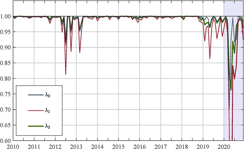
Note: the dotted blue line shows the cross-sectional correlation between the contemporaneous factor loadings $$\lambda_0$$ estimated on the sample ending at time $$t$$ and the $$\lambda_0$$ estimated on the sample ending at time $$t+1$$. The red (green) line shows the same statistics but for $$\lambda_1$$ ($$\lambda_2$$).
1. "M3" denotes the third month of the year. Return to text
2. ($$\hat{\chi}^c_t - \tilde{\chi}^c_t$$) is stationary because the data upon which the model is estimated are stationary. Moreover, because $$\xi^c_t$$ has by construction mean equal to zero, $$\hat{\chi}^c_t$$ and $$\tilde{\chi}^c_t$$ have the same mean, and therefore ($$\hat{\chi}^c_t - \tilde{\chi}^c_t$$) has sample mean equal to zero. Return to text
3. Since the PCE price index is a Fisher index it has the drawback of non-additivity property, hence only approximate weights can be computed (see footnote 5 in Luciani, 2020, and reference therein). Return to text
4. In the main text, I called $$\hat{\chi}^c_t$$ "the pattern of comovement during COVID," and $$\tilde{\chi}^c_t$$ "the stable pattern of comovement before COVID." Return to text
5. As shown in equation (2), the common component of price i, which captures the changes in inflation of price i that are common to all PCE prices, is obtained by multiplying the factors times the loadings. However, given a set of estimated parameters (and an initial condition), the factors are univocally determined, i.e., they can be expressed as a product of the data times the loadings and the other parameters—see for example Appendix A in Barigozzi and Luciani (2020). Therefore, the loadings are the main object that characterized the comovements in the data. Return to text
Luciani, Matteo (2021). "Quantifying the COVID-19 effects on core PCE price inflation," FEDS Notes. Washington: Board of Governors of the Federal Reserve System, Februray 25, 2021, https://doi.org/10.17016/2380-7172.2875.
Disclaimer: FEDS Notes are articles in which Board staff offer their own views and present analysis on a range of topics in economics and finance. These articles are shorter and less technically oriented than FEDS Working Papers and IFDP papers.