FEDS Notes
November 26, 2021
The Ability to Work Remotely: Measures and Implications
Kathryn Langemeier and Maria D. Tito1
At the onset of the COVID-19 recession, a large share of the employed switched to remote work. Individual- and firm-level surveys indicated that the switch affected between 35 and 45 percent of workers.2 The switch is even more remarkable if considering that, through early 2020, the share of people who worked from home across various surveys had remained remarkably stable.3 This recent pick-up in working from home could point to significant changes in the potential of remote work. This note explores how the ability to work remotely has changed over time, its relationship with demographic characteristics and employment outcomes, and the role it played during the pandemic recession.
In the recent literature, two contributions have proposed systematic approaches, based on occupation characteristics, aimed at identifying jobs that can be performed at home. Dingel and Neiman (2020) present a remote work index that looks extensively at work context and activities and flags, in particular, physical aspects of jobs—such as, physically dealing with aggressive people; being exposed to disease or infection; inspecting equipment, structure, or materials; etc.4 Because of this characterization, the remote work index proposed by Dingel and Neiman (2020) effectively captures occupations that can be performed at home because they require "no physical presence"—our preferred designation hereafter. Montenovo et al. (2020) describe a more concise index, focusing on email, phone, and memo usage; as such, we will refer to the Montenovo et al. (2020) measure as identifying occupations featuring "remote communications".5
The first objective of our note is to study the evolution of those measures. Using the definitions from Dingel and Neiman (2020) and Montenovo et al. (2020), we construct indexes of remote work from the Occupation Information Network (O*Net) questionnaires from July 2003 through February 2020. We then match those indexes with Bureau of Labor Statistics (BLS) data from the Current Population Survey (CPS) to measure the prevalence of remote work in overall employment.
Figure 1 describes the evolution of employment shares in remote occupations according to the no physical presence (left panel) and the remote communications (right panel) indexes. The two indexes present very different evolutions. While the no physical presence index has remained relatively constant, the remote communications index has gradually increased over time, gaining more than 40 percentage points in terms of employment shares relative to July 2003.6, 7 Looking at the more recent history, the discrepancies between the two indexes appear more contained. Occupations that require no physical presence represented about 42 percent of CPS employment in February 2020, while the share of employment in occupations characterized by remote communications was a little higher, reaching almost 50 percent before the pandemic recession.8
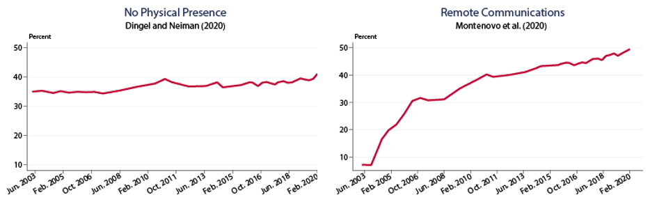
Notes: The left panel shows the share of employment in occupations that do not require physical presence. The right panel shows the share of employment in occupations with indices of e-mail, phone, and memo usage above 4.
Source: Bureau of Labor Statistics' Current Population Survey (CPS) and O*Net.
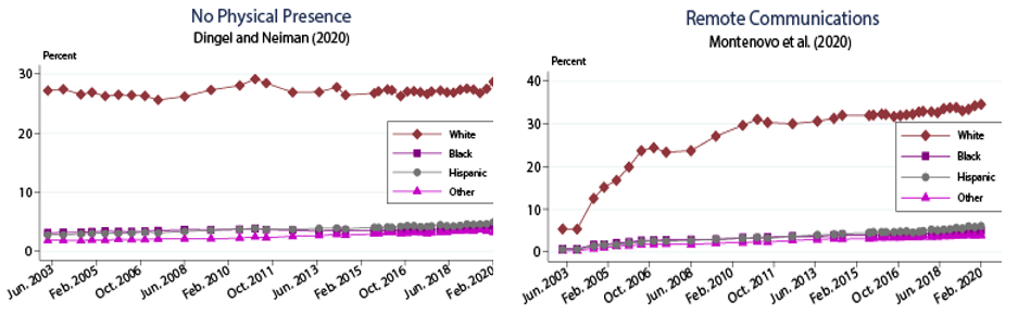
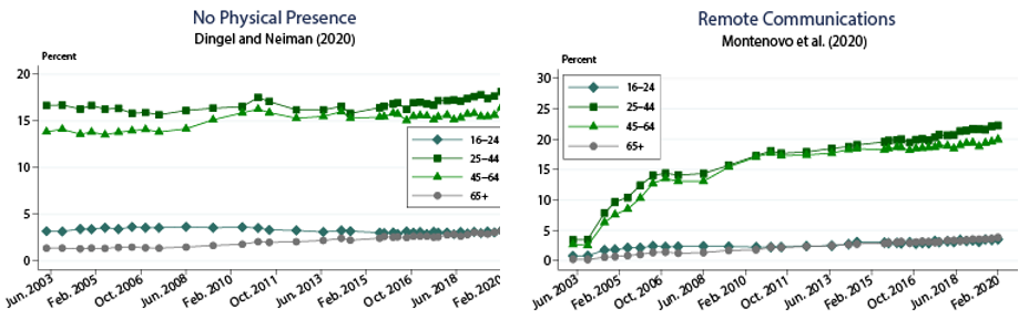
Next, we explore demographic correlates of remote work, extending the analysis by Mongey and Weinberg (2020). Figure 2 focuses on three main characteristics: race and ethnicity, age, and education level.9 The average distribution of remote work along these dimensions is consistent with the idea that highly teleworkable jobs tend to be in nonproduction/supervisory occupations, which are characterized by a disproportionately higher share of white employment (top panel) and require higher levels of education (bottom panel). Moreover, the prevalence of remote employment is more pronounced for those in the prime age group—that is, those between 25 and 64 years of age—while the share of remote jobs is more limited for those outside of that age range. We also looked at employment shares in remote occupations by gender, where the likelihood of men and women to be in a remote job appears fairly close. All told, the average disparities across demographic groups are relatively similar for each measure.
Employment Share by Race and Ethnicity
Employment Share by Age
Employment Share by Education Level
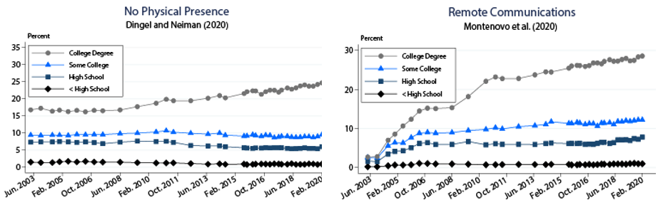
Notes: The left panels shows employment shares in occupations that do not require physical presence. The right panels shows employment shares in occupations characterized by a hight ability of working remotely, that is, by indices of e-mail, phone, and memo usage above 4. In panel A, other denotes Asian, American Indian or Alaska Native, and Native Hawaiian or Other Pacific Islander.
Source: BLS CPS and O*Net.
Focusing on changes in remote employment shares across those dimensions, the static nature of the aggregate no physical presence index transpires across all demographic groups except for college-educated workers. For the remote communications index, the group that represented the largest share of remote employment in 2003—white, 25-to-64, college-educated—grew at a steady pace over time, while the share of remote jobs in all other groups remained at consistently low levels. Naturally, differential trends in remote work across demographic groups could reflect many different factors—such as the increase in the pool of college-educated workers or a shift towards supervisory occupations—in addition to worker selection into remote occupations.
Beside the variation associated with demographic characteristics, occupations with the ability to work remotely also differ in terms of labor market outcomes: Table 1 explores differences in employment status, while figure 3 and table 2 highlight differences in wages. In both tables, columns (1)-(3) refer to the no physical presence index, while columns (4)-(6) characterize the results for occupations characterized by remote communications. Looking at the results in table 1, we find that people in occupations with the ability to work from home by either measure are less likely to be unemployed. The magnitude of the effect is slightly lower after controlling for worker observables—including demographic characteristics highlighted above—in columns (2) and (5), and a large set of fixed effects—state-year, industry-year, and month—in columns (3) and (6), but the coefficients continue to imply significant differences.
Table 1: Remote Work and Unemployment Probability
| (1) | (2) | (3) | (4) | (5) | (6) | |
|---|---|---|---|---|---|---|
| Variables | $${Unemployed}_t$$ | |||||
| No $${Physical\ Presence}_t$$ | -0.020*** | -0.007** | -0.006* | |||
| (0.004) | (0.003) | (0.003) | ||||
| $${Remote\ Comm}_t$$ | -0.033*** | -0.017*** | -0.017*** | |||
| (0.004) | (0.003) | (0.003) | ||||
| Worker Observables | n | y | y | n | y | y |
| Month FE | n | n | y | n | n | y |
| State-Year FE | n | n | y | n | n | y |
| Industry-Year FE | n | n | y | n | n | y |
| Obs. | 55,485 | 55,485 | 55,485 | 2,008,383 | 2,008,383 | 2,008,383 |
| R-squared | 0.003 | 0.023 | 0.027 | 0.009 | 0.032 | 0.039 |
$${Unemployed}_t$$: indicator equal to 1 if unemployed at time $$t$$.
$${Physical\ Presence}_t$$: indicators equal to 1 for occupations that do not require physical presence.
$${Remote\ Comm}_t$$: indicator equal to 1 for occupations that require high use of e-mails, memos, and telephone.
Legend: *** denotes significance at 1 percent level, ** significance at 5 percent, and * significance at 10 percent.
Notes: Cross-sectional regressions. Columns (2)-(3) and (5)-(6) include worker observables (age, gender, race, ethnicity, education, marital status, citizenship, tenure, and metro dummies); columns (3) and (6) also add month, state-year, and industry-year fixed effects. Robust standard errors, clustered at the occupation level, are reported in parenthesis.
Source: BLS CPS and O*Net.
Figure 3 points to large aggregate differences in average wages across remote and non-remote occupations by either index. Those who are able to work remotely have higher annual wage outcomes, with some slight differences across the indexes. Among those differences, the remote communications index shows a persistently wider gap than the no physical presence index, partly reflecting very anemic growth in non-remote workers' wages for the former measure.
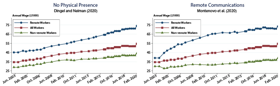
Notes: The left panel shows annual wage based on shares of employment in remote occupations using the Dingel and Neiman (2020) classification; the right panel shows annual wage based on shares of employment in remote occupations using the Montenovo et al. (2020) classification, above 80.
Source: BLS Occupational Employment Statistics and O*Net.
To control for the variation in hours across occupations, table 2 summarizes the variation in hourly wages across remote and non-remote jobs. The "remote" wage premium remains significant after including worker observables and fixed effects in our regressions. Using the specifications in columns (3) and (6), we find that a worker in an occupation that require no physical presence receives a 15 percent of a standard deviation (sd) higher hourly wage, while those employed in occupations characterized by remote communications enjoy a 35 percent of a sd higher hourly wage.10
Table 2: Remote Work and Wage Effects
| (1) | (2) | (3) | (4) | (5) | (6) | |
|---|---|---|---|---|---|---|
| Variables | $${Log\ Hourly\ Wage}_t$$ | |||||
| No $${Physical\ Presence}_t$$ | 0.341*** | 0.137*** | 0.100*** | |||
| (0.061) | (0.041) | (0.038) | ||||
| $${Remote\ Comm}_t$$ | 0.516*** | 0.273*** | 0.224*** | |||
| (0.054) | (0.038) | (0.035) | ||||
| Worker Observables | n | y | y | n | y | y |
| Month FE | n | n | y | n | n | y |
| State-Year FE | n | n | y | n | n | y |
| Industry-Year FE | n | n | y | n | n | y |
| Obs. | 11,672 | 11,672 | 11,672 | 419,389 | 419,389 | 419,389 |
| R-squared | 0.065 | 0.334 | 0.374 | 0.154 | 0.366 | 0.415 |
$${Log\ Hourly\ Wage}_t$$: hourly wage, in log-s, at time $$t$$.
$${Physical\ Presence}_t$$: indicators equal to 1 for occupations that do not require physical presence.
$${Remote\ Comm}_t$$: indicator equal to 1 for occupations that require high use of e-mails, memos, and telephone.
Legend: *** denotes significance at 1 percent level, ** significance at 5 percent, and * significance at 10 percent.
Notes: Cross-sectional regressions. Columns (2)-(3) and (5)-(6) include worker observables (age, gender, race, ethnicity, education, marital status, citizenship, tenure, and metro dummies); columns (3) and (6) also add month, state-year, and industry-year fixed effects. Robust standard errors, clustered at the occupation level, are reported in parenthesis.
Source: BLS CPS and O*Net.
The variation of employment outcomes for remote relative to other occupations underscores the scope of a role for remote work during the most recent recession. To more precisely understand the part that the switch to working remotely played in the past recession, we look at two pieces of evidence. First, we repeat the analysis in table 1 and 2 with remote indexes that reflect the February 2020 occupation characteristics. With a fixed classification of remote jobs, the correlation with employment outcomes will not be driven by shifts across occupations or changes in tasks within occupation. Furthermore, we'll disentangle a baseline impact of remote work on employment outcomes from the effect during the pandemic using an interaction between our indexes and an indicator variable equal to one during March and April 2020.
Our results for the first part of the analysis are shown in tables 3 and 4. Our indices of remote work based on the February 2020 characteristics are generally associated with a lower probability of unemployment and higher wages over the entire sample. In addition, during the pandemic recession, workers in remote occupations by either measure were even less likely to be unemployed but did not enjoy any additional wage gains.
Table 3: Remote Work and Probability of Being Unemployed during the Pandemic
| (1) | (2) | (3) | (4) | (5) | (6) | |
|---|---|---|---|---|---|---|
| Variables | $${Unemployed}_t$$ | |||||
| No $${Physical\ Presence}_t$$ | -0.029*** | -0.012** | -0.006 | |||
| (0.007) | (0.005) | (0.005) | ||||
| No $${Physical\ Presence}_t$$ * $${Pandemic}_t$$ | -0.018*** | -0.018*** | -0.014*** | |||
| (0.005) | (0.005) | (0.004) | ||||
| $${Remote\ Comm}_t$$ | -0.054*** | -0.039*** | -0.035*** | |||
| (0.006) | (0.005) | (0.005) | ||||
| $${Remote\ Comm}_t$$ * $${Pandemic}_t$$ | -0.030*** | -0.031*** | -0.027*** | |||
| (0.005) | (0.005) | (0.005) | ||||
| Worker Observables | n | y | y | n | y | y |
| Month FE | n | n | y | n | n | y |
| State-Year FE | n | n | y | n | n | y |
| Industry-Year FE | n | n | y | n | n | y |
| Obs. | 866,974 | 866,974 | 866,974 | 865,731 | 865,731 | 865,731 |
| R-squared | 0.004 | 0.037 | 0.059 | 0.013 | 0.042 | 0.063 |
$${Unemployed}_t$$: indicator equal to 1 if unemployed at time $$t$$.
$${Physical\ Presence}_t$$: indicators equal to 1 for occupations that do not require physical presence.
$${Pandemic}_t$$: indicator equal to 1 for March and April 2020.
$${Remote\ Comm}_t$$: indicator equal to 1 for occupations that require high use of e-mails, memos, and telephone.
Legend: *** denotes significance at 1 percent level, ** significance at 5 percent, and * significance at 10 percent.
Notes: Cross-sectional regressions. Columns (2)-(3) and (5)-(6) include worker observables (age, gender, race, ethnicity, education, marital status, citizenship, tenure, and metro dummies); columns (3) and (6) also add month, state-year and industry-year fixed effects. Robust standard errors, clustered at the occupation level, are reported in parenthesis.
Source: BLS CPS and O*Net.
Table 4: Remote Work and Wages during the Pandemic
| (1) | (2) | (3) | (4) | (5) | (6) | |
|---|---|---|---|---|---|---|
| Variables | $${Log\ Hourly\ Wage}_t$$ | |||||
| No $${Physical\ Presence}_t$$ | 0.317*** | 0.120*** | 0.087** | |||
| (0.058) | (0.038) | (0.035) | ||||
| No $${Physical\ Presence}_t$$ * $${Pandemic}_t$$ | -0.006 | 0.003 | 0.003 | |||
| (0.012) | (0.010) | (0.010) | ||||
| $${Remote\ Comm}_t$$ | 0.468*** | 0.251*** | 0.225*** | |||
| (0.048) | (0.030) | (0.026) | ||||
| $${Remote\ Comm}_t$$ * $${Pandemic}_t$$ | -0.011 | 0.008 | 0.008 | |||
| (0.011) | (0.010) | (0.010) | ||||
| Worker Observables | n | y | y | n | y | y |
| Month FE | n | n | y | n | n | y |
| State-Year FE | n | n | y | n | n | y |
| Industry-Year FE | n | n | y | n | n | y |
| Observations | 182,335 | 182,335 | 182,335 | 182,051 | 182,051 | 182,051 |
| R-squared | 0.056 | 0.303 | 0.336 | 0.136 | 0.325 | 0.354 |
$${Log\ Hourly\ Wage}_t$$: hourly wage, in log-s, at time $$t$$.
$${Physical\ Presence}_t$$: indicators equal to 1 for occupations that do not require physical presence.
$${Pandemic}_t$$: indicator equal to 1 for March and April 2020.
$${Remote\ Comm}_t$$: indicator equal to 1 for occupations that require high use of e-mails, memos, and telephone.
Legend: *** denotes significance at 1 percent level, ** significance at 5 percent, and * significance at 10 percent.
Notes: Cross-sectional regressions. Columns (2)-(3) and (5)-(6) include worker observables (age, gender, race, ethnicity, education, marital status, citizenship, tenure, and metro dummies); columns (3) and (6) also add month, state-year and industry-year fixed effects. Robust standard errors, clustered at the occupation level, are reported in parenthesis.
Source: BLS CPS and O*Net.
The differential employment outcomes for remote occupations are also reflected in the patterns of hours associated to remote jobs during the recent pandemic. Figure 4 compares three outcomes: the trend in hours across all occupations, the trend in hours across jobs characterized by remote communications, and the trend across jobs requiring no physical presence. Consistent with the findings in table 3, remote occupations by either index experienced a significantly smaller decline over the two months of the pandemic recession; as a result, the rebound in hours for remote occupations appears more gradual, but the level of hours at occupations requiring no physical presence or characterized by remote communications remains above the level of hours at all jobs throughout the middle of 2021. Since differences in the patterns of hours for the two indexes are minimal, our evidence so far suggests that either measure is representative of the status of remote work in the post-pandemic period.
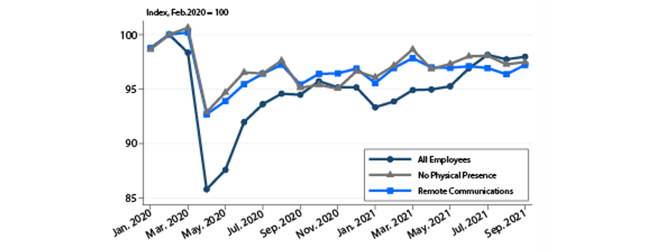
Notes: Decline in aggregate hours relative to February 2020. Remote communications refers to occupations with high usage of phone, e-mail, and memos; no physical presence refers to occupations that do not require physical presence.
Source: BLS CPS and O*Net.
In the second part of our analysis, we look at the counterfactual declines in hours in March and April 2020 had the ability of working remotely for each occupation remained at the same levels as in July 2004.11 Specifically, for each occupation with the ability to work remotely in February 2020 but not in July 2004, we attribute the average decline in hours of non-remote occupations over the recession period rather than the actual decline; we then look at the decline in total hours for this counterfactual scenario. The results for our exercise are shown in figure 5, with the left panel focusing on the index of no physical presence and the right panel displaying the effect for the index of remote communications.
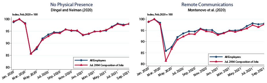
Notes: Decline in aggregate hours relative to February 2020. The left panel shows occupations that do not require physical presence. The right panel shows occupations with high use of phone, e-mail, and memos.
Source: BLS CPS and O*Net.
No changes in the ability of working remotely would have implied minimal effects in the hours decline observed in March and April 2020 for the index of no physical presence. The impact on hours, instead, would have been significantly more pronounced had the index of remote communications remained at the same level as that of July 2004. Table 5 summarizes our results and includes a comparison with the overall impact on hours and GDP in 2020.
Table 5. Working from Home: Impact on Hours
| 2020 | ||||
|---|---|---|---|---|
| Q1 | Q2 | Q3 | Q4 | |
| (1) Total Hours Decline (a.r.) Countefactuals as of Jul. 2004 | -3.6% | -36.5% | 25.8% | 7.2% |
| (2) No Physical Presence | -3.7% | -36.6% | 26.6% | 7.3% |
| (3) Remote Communications | -4.5% | -42.1% | 35.3% | 8.2% |
| (4) Memo: GDP growth (a.r.) | -4.9% | -31.3% | 33.6% | 4.5% |
Note: Total hours decline denotes the aggregate decline in usual hours. The counterfactual scenarios assume that occupations that could not performed at home in July 2004 by either measure experienced the same declines as non-teleworkable occupations in 2020 during the pandemic recession.
Source: BLS CPS,O*Net, and authors' calculations.
There are slight differences between the counterfactual scenario for the no physical presence index and the actual decline in hours, as shown in lines (1) and (2) of the table. For the remote communications index, instead, the increase in the ability of remote work prevented a further decline in hours of 0.9 percentage points (pp) in 2020Q1 and of 5.6 pp in 2020Q2. While the "remote communications" counterfactual points to a stronger rebound in hours starting in the third quarter, the level of the hours index for remote jobs based on the July 2004 data tracks a touch below the observed trend in hours.
All told, our analysis suggests that the ability of working remotely has had a meaningful impact on aggregate hours during the pandemic, although the effect could reflect either an increase in the ability of working remotely with the adoption of remote communications and or a switch to remote work for those occupations requiring no physical presence.
The significant decline in hours during the pandemic has affected the pattern of GDP growth, shown in line (4). Naturally, the divergence between hours and GDP growth reflects the impact of productivity growth, another important dimension in the analysis of the ability of working remotely. While the evidence on the effect of remote work on productivity is mixed, our results point to the significant contribution of the ability to work remotely to the hours margin.12 The two indexes display a very different evolution in how many jobs can be performed at home. However, either because our ability to work remotely has significantly increased over the past two decades or because the pandemic has prompted an acceleration towards telecommuting, the resulting gains in hours from remote work will likely persist, contributing to a higher level of GDP.
References
Bartik, A. W., Z. B. Cullen, E. L. Glaeser, M. Luca, and C. T. Stanton (2020), "What jobs are being done at home during the Covid-19 crisis? Evidence from firm-level surveys", NBER Working Paper n. 27422.
Bloom, N., J. Liang, J. Roberts and Z. J. Ying (2015), "Does working from home work? Evidence from a Chinese experiment", Quarterly Journal of Economics, Vol. 130, pag. 165–218.
Bureau of Labor Statistics (2020), "Current Population Survey", available at https://www.census.gov/programs-surveys/cps/data/datasets.html
Bureau of Labor Statistics (2020), "Occupational Employment Statistics", available at https://www.bls.gov/oes/tables.htm
Brynjolfsson E., J.J. Horton, A. Ozimek, D. Rock, G. Sharma, and H.Y. TuYe (2020), "COVID-19 and remote work: an early look at US data", NBER Working Paper n. 27344.
Dingel, J. and B. Neiman (2020), "How many jobs can be done at home?", Journal of Public Economics, Vol. 189.
Mas, A. and A. Pallais (2020), "Alternative work arrangements", Annual Review of Economics, Vol. 12, pag. 631–658.
Mongey, S. and Weinberg, A. (2020). Characteristics of workers in low work-from-home and high personal-proximity occupations. Becker Friedman Institute for Economic White Paper.
Montenovo L., X. Jiang, F.L. Rojas, I.M. Schmutte, K.I. Simon, B.A. Weinberg, and C. Wing (2020), "Determinants of disparities in COVID-19 job losses", NBER Working Paper n. 27132.
Morikawa, M. (2020), "Productivity of working from home during the COVID-19 pandemic: Evidence from an employee survey", Covid Economics, Vol. 49, pag. 123–139.
Occupation Information Network Center, (2020) O*Net Database, available at https://www.onetcenter.org/database.html.
1. The views expressed in the article are those of the authors and do not necessarily reflect those of the Federal Reserve System. We would like to thank John Roberts for his insightful comments. Return to text
2. See, for example, Bartik et al. (2020) and Brynjolfsson et al. (2020) Return to text
3. See Mas and Pallais (2020). Return to text
4. In Dingel and Neiman (2020), a job cannot be performed at home if either the average respondent indicates that he/she uses e-mail less than once a month; is physically dealing with aggressive people; is exposed to disease, infections, minor burns, cuts, bites, or stings; works outdoor every day; wears specialized or common protective equipment; spends time walking and running; or if it is very important to perform physical activities; to handle or move objects; to control machine and processes; to operate vehicles or mechanized devices; to perform or work directly with the public; to inspect equipment, structures, or material; to repair and maintain electronic or mechanical equipment. Return to text
5. In Montenovo et al. (2020), a job is flagged as "remote" if e-mail, phone, or memo usage is very important. Return to text
6. Using the Occupational Employment Statistics (OES) data, which covers 200,000 establishments—compared with about 4,500 household interviews for CPS—the remote communications index has grown from 9.8 million in 2003 to 57.7 million workers in February 2020; the no physical presence has, instead, grown only from 39.5 million to 44.5 million workers. Our analysis relies on CPS because of the availability of worker observable characteristics. Return to text
7. The gradual evolution of remote work observed in the remote communications measure appears more aligned with the behavior of other measures. In particular, the CPS Supplement data indicate that, in 2004, the share of remote employment was 15 percent compared with 16.5 percent for the remote communications index and 34.6 percent for the no physical presence index. Return to text
8. Dingel and Neiman (2020) match the remote index with the OES data and estimate that, using the February 2020 O*Net survey, 37 percent of jobs could be performed at home according to their definition. Return to text
9. The figure decomposes the contribution of each group to the total share of employment in remote occupations by either measure. Return to text
10. In our sample, one standard deviation of log hourly wages is 0.65. Return to text
11. We chose July 2004 as a reference period to match our comparison with the CPS supplement data on remote work for that year. Using data from April 2003, our results for the no physical presence measure would be little changed, while the counterfactual for the remote communications index would imply larger declines. Return to text
12. The seminal work by Bloom at al. (2015) point to productivity gains associated with remote work since it would allow workers to better organize business and home tasks. Yet, using Japanese survey data, Morikawa (2020) finds that productivity in June 2020 was only about 60% to 70% of what it was in the workplace in June 2019. Return to text
Langemeier, Kathryn, and Maria D. Tito (2021). "The Ability to Work Remotely: Measures and Implications," FEDS Notes. Washington: Board of Governors of the Federal Reserve System, November 26, 2021, https://doi.org/10.17016/2380-7172.3032.
Disclaimer: FEDS Notes are articles in which Board staff offer their own views and present analysis on a range of topics in economics and finance. These articles are shorter and less technically oriented than FEDS Working Papers and IFDP papers.