Board of Governors of the Federal Reserve System

Thank you very much for inviting me to be part of the H. Parker Willis Lecture Series. As you know, Dr. Willis was a distinguished professor here at Washington and Lee University. Among many other accomplishments, he helped create the Federal Reserve System. He served as the first secretary to the Federal Reserve Board from 1914 to 1918 and later as the first research director.

Before I go further, let me remind you that the views I will express today are my own and are not necessarily those of my colleagues in the Federal Reserve System.

Many discussions of monetary policy simply talk about the Federal Reserve setting the federal funds rate to promote our goals of maximum employment and price stability, without giving attention to the specific actions we take to put the federal funds rate where we want it—that is, to the way we implement monetary policy. And even in economics classes that cover this topic, the teaching materials have not always caught up with the fact that we have purposely changed our implementation framework over the past decade.¹ My colleagues at the Fed are working with educators to close the curriculum gap, and I hope this lecture will further help this endeavor.²

In honor of Dr. Willis's important contributions to the design and creation of the Federal Reserve, today I would like to talk to you about how the Fed currently uses a specific set of tools to implement monetary policy and how monetary policy is transmitted to the economy. Then, I will offer some concluding remarks.

The Federal Funds Market and the Fed's Policy Target Range
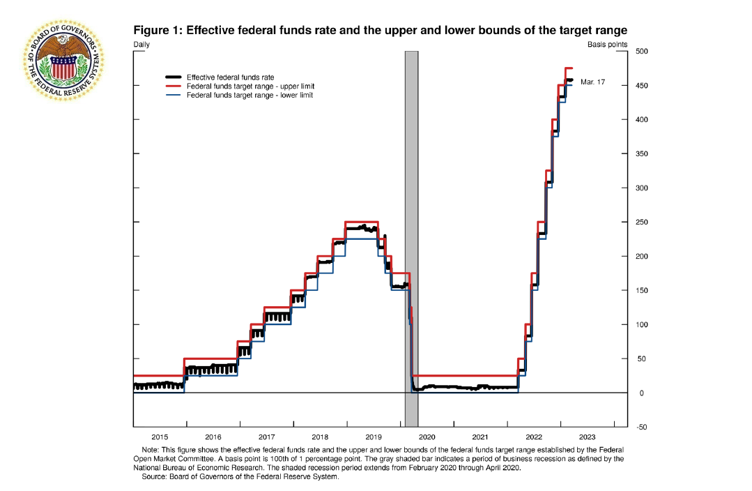
As mandated by the U.S. Congress, the Federal Open Market Committee's (FOMC) objectives are to promote maximum employment and price stability. The members of the Board of Governors and the presidents of the 12 Federal Reserve Banks constitute the FOMC. The FOMC gathers for eight regularly scheduled meetings each year to discuss economic and financial conditions and to deliberate on monetary policy. In each meeting, the FOMC establishes a target range for the federal funds rate. Figure 1 shows the upper bound in red and the lower bound in blue of the federal funds target range since 2015. We see the range increasing in 2018 as the job market was strengthening and inflation was moving up toward 2 percent. That's right—for much of the decade before then, the inflation rate was below 2 percent. In March 2020, when the COVID-19 pandemic hit the economy, the FOMC quickly moved the target range down to near zero to support economic activity.

Once monetary policy is set, the Fed implements monetary policy by using its policy tools to ensure that the federal funds rate (FFR) stays within the range. The effective federal fund rate is determined by market forces. It is a volume-weighted median of federal funds rates across all borrowers each day. In figure 1, you can see that the Fed has been able to implement monetary policy in such a way that the effective federal funds rate (EFFR), the black line in the figure, has indeed stayed within the target rate range most of the time.

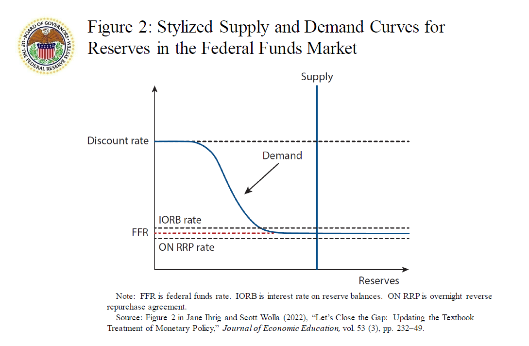
To understand how the Fed's tools work, it is important to understand the federal funds market. It is a market where depository institutions borrow funds overnight from certain financial institutions, including other depository institutions and government-sponsored enterprises. These loans are uncollateralized, and the interest rate or cost of the loans is the federal funds rate, which is determined by the supply and demand for reserve balances that financial institutions hold in their "checking accounts" at the Fed.³ The Fed can change the total amount of reserves available to the banking system through open market operations or its lending programs. Since the Fed controls the supply of reserves and the amount that it supplies is independent of the interest rate, the supply of reserves is illustrated as a vertical line in the stylized supply and demand curves shown in figure 2.⁴ Later, I will explain why this supply curve intersects the demand curve, as shown in figure 2.

The demand curve for reserves in figure 2 has three segments. The top portion of the demand curve is capped by the discount rate that the Fed sets. The middle of the curve is downward sloping, like most demand curves. The higher the interest rate or cost to borrow, the lower the quantity of reserves demanded. The bottom portion is nearly flat because, at some point, banks do not find much benefit from holding additional reserves other than earning the interest on reserve balances (IORB) rate from the Fed. In other words, banks prefer to earn money by making loans to consumers and businesses or purchasing securities only if doing so generates a higher return. In what follows, I will go deeper into the top and bottom segments of the demand curve.

Implementation Tool 1: Discount Window Rate Sets a Ceiling
At the top of the demand curve, we see the discount rate, which is the interest rate the Fed charges when it lends money to banks.⁵ The discount rate is an administered rate, or a rate set by the Fed, and it is one of the tools the Fed uses to implement monetary policy. It sets a ceiling for the federal funds rate because banks, if they are in good standing and have collateral for the discount window loan, can always borrow overnight funds at the discount rate from the Fed. Therefore, they are not willing to pay a higher rate to borrow funds.

In practice, however, banks have demonstrated, in the absence of stress, some reluctance to borrow from the discount window. They are concerned that borrowing from the Fed may indicate that the bank is unable to borrow from other financial institutions, and that it sends a negative signal about their financial condition to the world.⁶ Such dynamics are referred to as the "stigma" associated with the use of the discount window.⁷ Stigma dampens the discount rate's effectiveness as a day-to-day tool the Fed can use to implement monetary policy. Thus, alternative implementation tools are required. This brings me to the next rate I want to talk to you about, the interest rate on reserve balances.

Implementation Tool 2: Interest on Reserve Balances
Close to the bottom of the demand curve is the interest on reserve balances rate denoted by IORB rate in figure 2. This is the interest rate the Fed pays on reserves eligible institutions keep at Federal Reserve Banks.⁸ This interest rate is the primary tool the Fed uses currently to implement monetary policy.⁹ In the graph, observe that the federal funds rate is close to this rate. The economic force that keeps these two rates close to each other is called arbitrage, the simultaneous purchase and sale of funds (or goods) to profit from a difference in price. Arbitrage keeps prices of financial instruments with similar payoffs close to each other.¹⁰ I will illustrate how arbitrage works with an example that makes it clear why the federal funds rate cannot be much lower nor much higher than the interest on reserve balances rate.

Arbitrage Keeps Rates Close to Each Other
Let's assume that the federal funds rate is 4 percent and the interest on reserves is 4.5 percent. Banks will quickly realize that they can borrow funds in the federal funds market at 4 percent and deposit those funds at the Fed and earn the interest on reserve balances rate of 4.5 percent, which means that they can earn a profit of 0.5 percent (the difference between the two rates).¹¹ This riskless investment strategy is called an arbitrage opportunity. As long as this arbitrage opportunity exists, banks will borrow funds in the federal funds market and deposit those funds at the Fed, putting upward pressure on the federal funds rate. This upward pressure will continue until the federal funds rate rises to a level close to the interest on reserves and the arbitrage opportunity no longer exists.

A similar logic applies when the federal funds rate is much higher than the interest on reserves.¹² If this is the case, banks can make money by withdrawing funds from their "checking account" at the Fed and lending that money at the higher federal funds rate. More banks willing to lend money in the federal funds market will put downward pressure on the federal funds rate, causing the federal funds rate to decline toward the interest rate on reserves.

Implementation Tool 3: Overnight Reverse Repurchase Agreement
So far, I have talked about two of the Fed's administered rates; the discount rate, and the interest on reserve balances rate. Now, I will talk about the third key administered rate, the overnight reverse repurchase agreement rate denoted by ON RRP in figure 2. Not all institutions that lend money in the federal funds market and who are key players in short-term money markets are eligible to receive interest on reserves. Consider, for example, Federal Home Loan Banks. They were set up in the 1930s to support mortgage lending. Today, they manage about $1.5 trillion in assets. They are major lenders in the federal funds market, but they are ineligible to receive interest on reserves. Therefore, they may have an incentive to lend funds at a much lower rate than the interest rate on reserves rather than earn zero interest on idle cash balances. To ensure that these and other institutions do not charge an interest rate much lower than the interest rate on reserves, the Fed uses an overnight reverse repurchase agreement facility as a supplementary policy tool to help control the federal funds rate.¹³

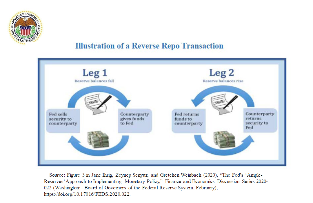
This facility is open to a broad set of financial institutions, including money market funds (MMFs), government-sponsored enterprises, and banks that are active in financial markets where short-term interest rates are determined. At this facility, institutions agree to buy a Treasury security from the Fed and sell it back the next day. In return, the Fed pays the institution the overnight reverse repurchase rate.¹⁴ Even though this transaction seems complicated, it is similar to banks depositing reserves at the Fed and receiving interest on them. This transaction, illustrated on slide 5, is equivalent to financial institutions depositing cash at the Fed and the Fed giving them a Treasury security as collateral, paying them the overnight reverse repurchase rate on the deposit, and agreeing to buy back the security the next day.

This facility sets a floor for the federal funds rate because not only banks, but other financial institutions can always earn the overnight reverse repurchase agreement rate when lending money to the Fed.¹⁵ In other words, the interest rate at this facility serves as a reservation rate, or the lowest rate lenders are willing to accept for lending out their cash.

Ample Reserves
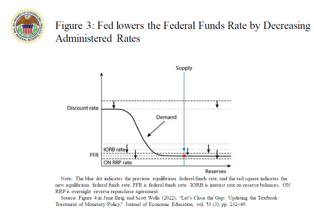
As I mentioned earlier, the federal funds rate is determined by borrowers and lenders. In figure 3, it is the point where supply and demand intersect. In this figure, notice that the supply curve is off to the right and it intersects the flat part of the demand curve. This is on purpose because we are currently in what we call an ample-reserves environment.¹⁶ In this environment, the Fed is supplying an "ample" level of reserves to the banking system, and small movements in the supply curve will not affect the equilibrium federal funds rate much. Instead, as I mentioned earlier, the key tool the Fed uses to implement monetary policy is the interest rate on reserves balances. In figure 3, you can see that by moving the interest rate on reserves down, the Fed shifts the demand for reserves down and affects the federal funds rate even if the demand curve is flat.¹⁷ A similar mechanism follows by moving the rate up. As suggested by the graph, the FOMC is mindful about adjusting its other administered rates in sync with the interest rate on reserve balances. This practice helps ensure arbitrage works to shift the demand curve as indicated.

Implementation Tool 4: Open Market Operations
So far, I have talked about how the Fed influences the demand curve by changing its administered rates. Now, I will talk about how the Fed shifts the supply of reserves in the system. It does so by buying or selling securities, so-called open market operations. When the Fed purchases securities, it pays for them by depositing cash into the appropriate banks' reserve balance accounts, adding to the overall level of reserves (cash) in the banking system.

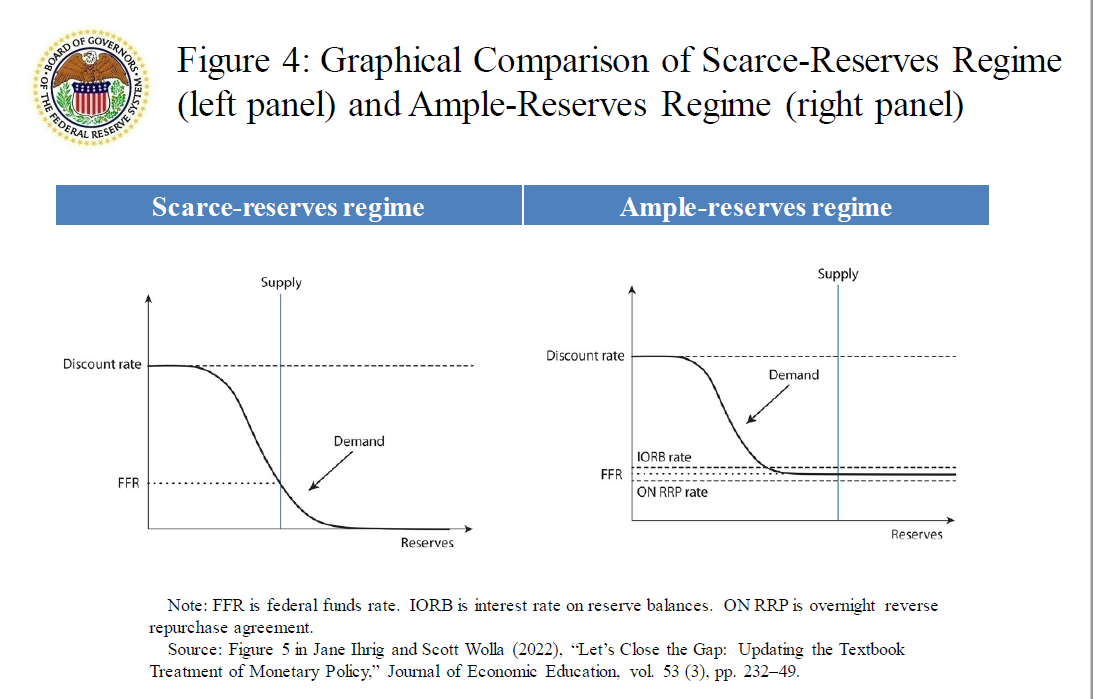
Before 2008, open market operations were the Fed's primary monetary policy tool because there were limited reserves in the banking system, a so-called scarce-reserves regime. In a scarce-reserves environment, the supply curve intersects the demand curve on the downward-sloping part of the demand curve, as illustrated in the left panel of figure 4. Open market operations are the tool old textbooks emphasize. The Fed would inject or drain reserves through open market operations to keep the vertical supply curve at the desired location—where it intersects the demand curve at the intended federal funds rate. Since the supply of reserves naturally changes—for example, because of the withdrawal of reserves into physical currency—the Fed conducted these operations frequently. Today, being in an ample-reserves regime, the Fed operates on a different segment of the demand curve and uses different tools, as illustrated in the right panel of figure 4.

Technical Adjustments to the Supply of Reserves: A Case Study
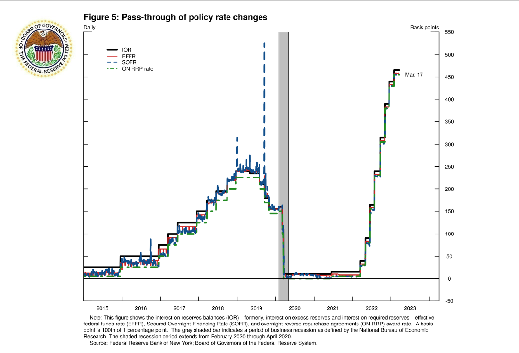
Although active management of the supply of reserves is not, by design, a feature of an ample-reserves regime, there are times when the Fed may take steps to adjust the supply of reserves to support interest rate control. For example, in mid-September 2019, strains in funding markets emerged as quarterly corporate tax payments and the settlement of Treasury securities coincided and resulted in a large amount of cash being drained from short-term interest rate investments. In fact, reserve balances fell more than $100 billion over just two days. Although the drain in reserves associated with seasonal tax payments was expected to put some upward pressure on short-term interest rates, the increases in rates that materialized were exceptionally large by historical standards. One such interest rate is the Secured Overnight Financing Rate, a broad measure of the cost of borrowing cash overnight collateralized by Treasury securities. As shown in figure 5, the blue dashed line denoted as SOFR spiked, and the effective federal funds rate, the red solid line, moved 5 basis points above the target range during this episode.

In response to these market developments the Fed undertook open market operations to purchase securities to add reserves temporarily. Specifically, the Fed conducted repurchase agreement (repo) transactions to provide immediate liquidity to the market and help alleviate the funding strains, ensuring the federal funds rate resumed trading within the target range. In addition, the FOMC judged that the prevailing level of reserve supply at that time may have been a bit too low to be consistent with operating in an ample-reserves regime. Accordingly, in early October 2019, the FOMC directed the Fed to maintain over time reserve balances at least as large as the level that had prevailed in "early September," a time when there were no evident pressures in money markets.¹⁸

The Fed's Balance Sheet
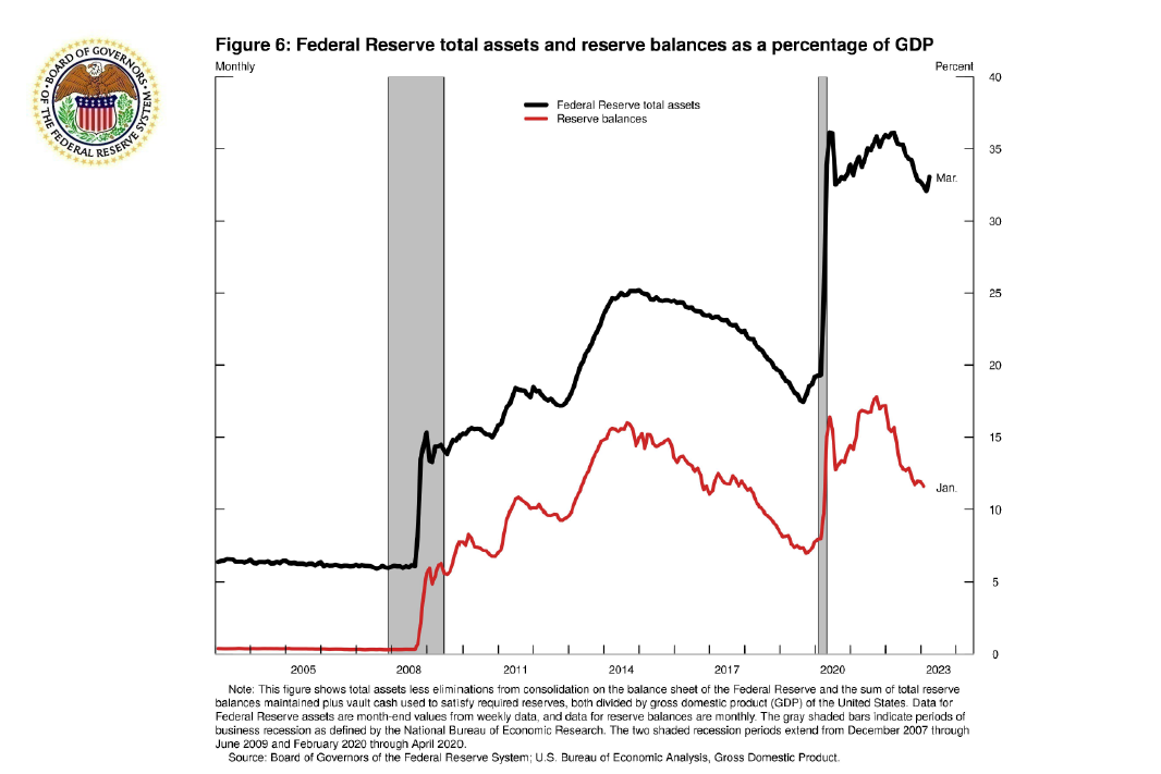
The Fed's balance sheet contains a great deal of information about the scale and scope of its open market operations. Figure 6 shows the evolution of the Fed's balance sheet, where the holdings of U.S. Treasury securities, agency mortgage-backed securities (MBS), and other securities are recorded as assets and reserve balances are recorded as liabilities. Both series are divided by gross domestic product because the Fed's balance sheet should naturally increase over time with economic growth. We entered the ample-reserves regime in 2008, during the 2007–09 financial crisis, as the Fed sharply increased its total assets. In 2020, during the COVID-19 pandemic, there was another sharp increase in total assets. In both instances, the Fed reduced its interest rate target near zero and purchased securities, injecting reserves into the banking system. The effect of purchasing securities was to reduce longer-term interest rates to support the economy. The expansion of the Fed's balance sheet is popularly known as quantitative easing (QE). When QE ended, the Fed reinvested any maturing securities it held to maintain the size of the balance sheet. Now, the Fed is fighting inflation by raising its interest rate target range and is in the process of shrinking the Fed's balance sheet, which is referred to as quantitative tightening (QT), by passively stopping the reinvestment in some maturing Treasury securities and agency mortgage-backed securities (MBS).¹⁹

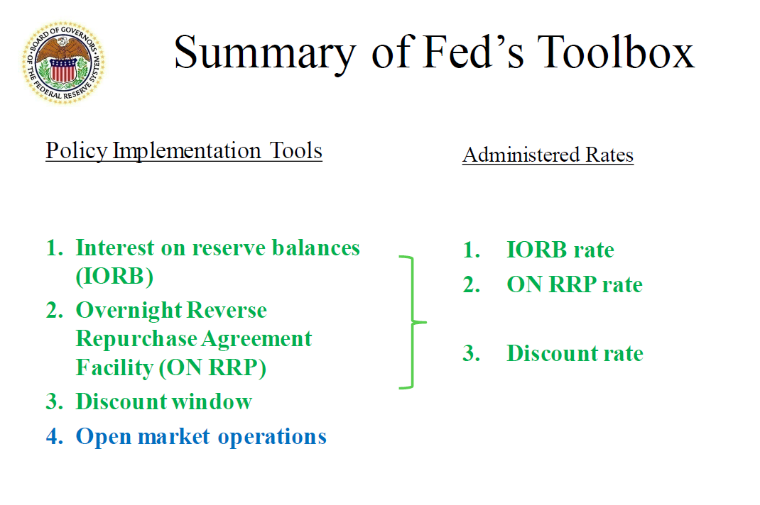
Summary of Tools
I've talked about how the Fed has four tools in its toolbox to implement monetary policy. Three of the tools and their associated administered rates, shown in green text on slide 10, are used to steer the market-determined federal funds rate into the FOMC's target range. These tools also interact with other short-term market interest rates through arbitrage relationships. The fourth tool, shown in blue text, is open market operations—the purchase and sale of government securities—which is used to adjust the supply of reserves in the banking system.

Monetary Policy Transmission
Now that you understand the Fed's implementation tools, let's see how the Fed uses them to achieve its two mandated goals: maximum employment and price stability. Currently, the unemployment rate is low, and the inflation rate is above the Fed's 2 percent target. Beginning in the second half of 2021, as the magnitude and persistence of the increase in inflation became clearer and as the job market recovery accelerated, the FOMC pivoted toward a tighter stance of monetary policy. In March 2022, the FOMC increased its target range for the federal funds rate, for the first time since the onset of the pandemic. In June 2022, we began the process of significantly reducing the size of our balance sheet, after announcing our plans in May.

Monetary policy is transmitted to the rest of the economy by affecting financial market prices, such as long-term interest rates, which in turn affect the decisions of households and businesses. Previously, I discussed how changes in the federal funds target range are transmitted to short-term interest rates, such as the overnight reverse repo rates, through arbitrage relationships. Short-term interest rates, in turn, affect long-term interest rates through investors' expectations. More specifically, according to the expectations theory of the term structure of interest rates, intermediate- and long-term interest rates are the weighted average of expected future short-term interest rates.²⁰ In addition, monetary policy affects risk premiums. Tighter monetary policy tends to reduce the willingness of investors to bear risk, making them less willing to invest in long-term assets, which means that their return (interest rate) must increase for investors to buy these assets.²¹

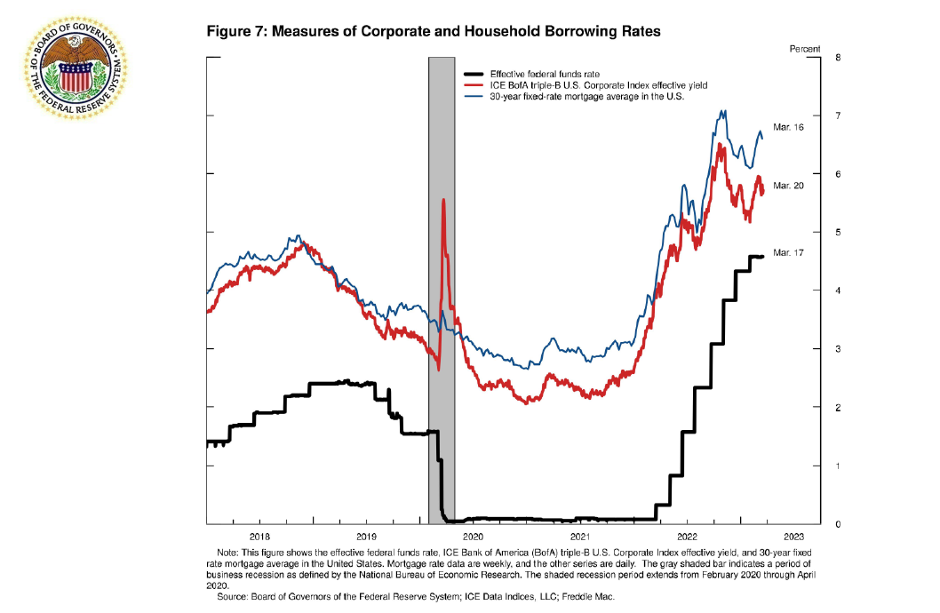
Figure 7 illustrates how long-term interest rates, which are widely viewed as important for businesses' and households' economic decisions, move in anticipation of changes in the federal funds rate. The red line is the average 10-year triple-B corporate bond rate. It is a measure of corporate borrowing costs. The blue line is the average 30-year mortgage rate. It is a measure of household borrowing costs. Notice that both measures increased in early 2022 in response to Fed communications and in anticipation of increases in the effective federal funds rate, the black line. Higher long-term interest rates increase the cost of borrowing money for households and businesses. Therefore, high interest rates raise the incentive to save, which in turn dampens consumer spending on interest rate-sensitive expenditures, like housing and automobiles, and slows businesses' investment in new equipment. The decrease in spending decreases the overall demand for goods and services in the economy, thereby reducing the demand/supply imbalances we have seen, and, consequently, reduce inflationary pressures. As a result, the inflation rate should fall back toward 2 percent, the FOMC's inflation rate target.

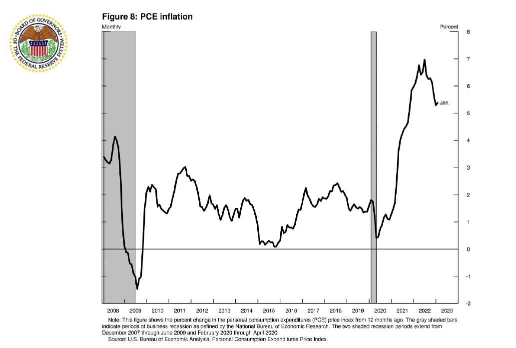
A key question is how much the tightening of financial conditions since late 2021 has contributed to reducing aggregate demand and inflationary pressures. In figure 8, you can see that inflation, measured using the personal consumption expenditures price index, has started to come down. Some of the disinflation, or reduction in the inflation rate, is due to monetary policy tightening, and some of this disinflation is due to other factors, such as supply chain bottlenecks easing and falling energy prices. Chair Powell and other colleagues in the Federal Reserve System have pointed out that monetary policy affects the economy and inflation with long, variable, and highly uncertain lags, and we are still learning about the full effect of our tightening thus far.²²

Conclusion
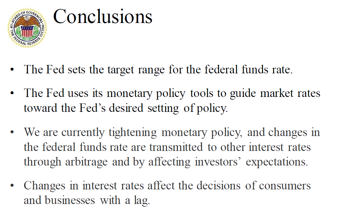
In conclusion, the Fed has a congressional mandate of maximum employment and price stability. The FOMC conducts monetary policy by setting the target range for the federal funds rate. Then, the Fed uses its monetary policy tools to implement the policy, which guides market interest rates toward the Fed's desired setting of policy. The Fed implements monetary policy using administered rates. The interest rate on reserve balances is the Fed's primary tool for adjusting the federal funds rate. The overnight reverse repurchase agreement facility is a supplementary tool that sets a floor for the federal funds rate. The discount rate serves as a ceiling for the federal funds rate. The Fed ensures that the banking system has ample reserves, using open market operations, if needed. Currently, we are tightening monetary policy. Changes in the federal funds rate are transmitted to other interest rates through arbitrage and by affecting investors' expectations. Changes in interest rates affect the decisions of consumers and businesses with a lag. Their decisions ultimately move the economy toward maximum employment and price stability.

Thank you.

References
Afonso, Gara, Domenico Giannone, Gabriele La Spada, and John C. Williams (2022). "Scarce, Abundant, or Ample? A Time-Varying Model of the Reserve Demand Curve," (PDF) Staff Report 1019. New York: Federal Reserve Bank of New York, May.

Bernanke, Ben S., and Kenneth N. Kuttner (2005). "What Explains the Stock Market's Reaction to Federal Reserve Policy?" Journal of Finance, vol. 60 (June), pp. 1221–57.

Board of Governors of the Federal Reserve System (2018). "Overnight Reverse Repurchase Agreement Facility," webpage, January 3.

——— (2019a). "Statement Regarding Monetary Policy Implementation and Balance Sheet Normalization," press release, January 30.

——— (2019b). "Statement Regarding Monetary Policy Implementation," press release, October 11.

——— (2022). "Discount Window Lending," webpage, December 30.

——— (2023). "Bank Term Funding Program," webpage, March 16.

Campbell, John Y., and John H. Cochrane (1999). "By Force of Habit: A Consumption-Based Explanation of Aggregate Stock Market Behavior," Journal of Political Economy, vol. 107 (April), pp. 205–51.

Carlson, Mark, and Jonathan D. Rose (2017). "Stigma and the Discount Window," FEDS Notes. Washington: Board of Governors of the Federal Reserve System, December 19.

Federal Reserve Bank of New York (2023). "FAQs: Reverse Repurchase Agreement Operations," webpage, February 22.

Gertler, Mark, and Peter Karadi (2015). "Monetary Policy Surprises, Credit Costs, and Economic Activity," American Economic Journal: Macroeconomics, vol. 7 (January), pp. 44–76.

Hanson, Samuel G., and Jeremy C. Stein (2015). "Monetary Policy and Long-Term Real Rates," Journal of Financial Economics, vol. 115 (March), pp. 429–48.

Ihrig, Jane, and Scott Wolla (2022a). Interview by Adrian Ma and Darian Woods, "AP Macro Gets a Makeover," The Indicator from Planet Money, NPR, August 15.

Ihrig, Jane, and Scott Wolla (2022b). "Let's Close the Gap: Updating the Textbook Treatment of Monetary Policy," Journal of Economic Education.

Ihrig, Jane, Zeynep Senyuz, and Gretchen C. Weinbach (2020). "The Fed's 'Ample Reserves' Approach to Implementing Monetary Policy," Finance and Economics Discussion Series 2020-022. Washington: Board of Governors of the Federal Reserve System, February (revised March 2020).

King, Robert G., and André Kurmann (2002). "Expectations and the Term Structure of Interest Rates: Evidence and Implications," Federal Reserve Bank of Richmond, Economic Quarterly, vol. 88 (Fall), pp. 49–95.

Lopez-Salido, David, and Annette Vissing-Jorgensen (2023). "Reserve Demand, Interest Rate Control, and Quantitative Tightening," Working Paper.

Piazzesi, Monika, and Martin Schneider (2006). "Equilibrium Yield Curves," NBER Working Paper Series 12609. Cambridge, Mass.: National Bureau of Economic Research, October (revised January 2007).

---

1. See the NPR interview with Jane Ihrig and Scott Wolla (2022a). Return to text

2. Some of the teaching materials that Jane Ihrig and Scott Wolla have created to close the curriculum gap are available on the Federal Reserve Bank of St. Louis's website at https://www.stlouisfed.org/education/teaching-new-tools-of-monetary-policy. For more information, please see Ihrig and Wolla (2022b). Return to text

3. An uncollateralized or unsecured loan is a loan that does not require any type of collateral. In contrast, a collateralized or secured loan is a loan that is backed by collateral, meaning something the borrower owns (collateral), such as U.S. Treasury securities, can be taken by the lender in case the borrower does not pay back the loan under the agreed terms. Return to text

4. The Fed understands that several factors affect the supply of reserves and that it can choose what operations to take, if any, in response. As a result, one should think of the Fed as controlling the supply of reserves in the banking system. For a detailed discussion of supply and demand of reserves, see Ihrig, Senyuz, and Weinbach (2020). Return to text

5. Depository institutions have access to three types of discount credit from their regional Federal Reserve Bank: primary credit, secondary credit, and seasonal credit, each with its own interest rate. We use the term "discount rate" as a shorthand for primary credit rate. Most credit at the discount window is done at the primary credit rate. For more information, please refer to Board of Governors (2022). Return to text

6. The list of banks that borrow money from the discount window is published with a two-year delay. Discount window borrowing increased recently following the failure of Silicon Valley Bank and Signature Bank. On March 12, 2023, the Fed announced a Bank Term Funding Facility to complement the funding available at the discount window; see Board of Governors (2023). Return to text

7. For a detailed discussion about the stigma associated with discount window borrowing, please see Carlson and Rose (2017). Return to text

8. Section 19(b)(2) of the Federal Reserve Act requires each depository institution to maintain reserves against certain liabilities of the bank. The Board's Regulation D (Reserve Requirements of Depository Institutions in title 12, part 204, of the Code of Federal Regulations) implements the reserve requirements provisions in section 19. Eligible institutions include depository institutions and certain other institutions as specified in the act; see the definition in 12 C.F.R. § 204.2 at https://www.ecfr.gov/current/title-12/chapter-II/subchapter-A/part-204/section-204.2#p-204.2(y). Return to text

9. On October 6, 2008, the Fed started to pay interest on reserves of eligible institutions with master accounts at Federal Reserve Banks. Up to and including July 28, 2021, interest was paid on required reserves at an IORR (interest on required reserves) rate and at an IOER (interest on excess reserves) rate. The IORR rate was paid on balances maintained to satisfy reserve balance requirements, and the IOER rate was paid on excess balances. Effective March 24, 2020, the Board amended Regulation D to set all reserve requirement ratios for transaction accounts to 0 percent, eliminating all reserve requirements. As a result, there is no longer a need to describe interest rates based on whether the balance satisfies a reserve balance requirement. To account for those changes, the Board approved a final rule amending Regulation D to replace references to an IORR rate and to an IOER rate with references to a single IORB rate. Return to text

10. This idea is called the law of one price, and it assumes that markets are competitive—that is, investors cannot manipulate prices to their advantage—and the absence of trade restrictions and trading costs. Return to text

11. This profit calculation assumes operational and regulatory costs are zero. Return to text

12. For the arbitrage strategies described earlier to work, the system needs to have sufficient reserves and enough competition among banks. Return to text

13. The Fed introduced the ON RRP facility in September 2013 and conducted test operations through late 2015. In September 2014, the FOMC indicated that it intended to use the facility as needed to help control the federal funds rate. For more information, see Board of Governors (2018) and Federal Reserve Bank of New York (2023). Return to text

14. The interest rate that a counterparty receives is the facility's offering rate except in the highly unlikely event that the amount of propositions the Fed receives exceeds the amount of securities available for the operation. In that case, the interest rate would be determined by an auction process conducted by the Federal Reserve Bank of New York, as described in Federal Reserve Bank of New York (2023). Return to text

15. For banks eligible to receive the IORB rate, the IORB rate is their reservation rate, and it explains why the federal funds market is currently dominated by nonbank lenders with the EFFR remaining below the IORB rate. Return to text

16. In January 2019, the Fed announced that "the Committee intends to continue to implement monetary policy in a regime in which an ample supply of reserves ensures that control over the level of the federal funds rate and other short-term interest rates is exercised primarily through the setting of the Federal Reserve's administered rates, and in which active management of the supply of reserves is not required." See Board of Governors (2019a, para 2). Afonso and others (2022), among others, investigate how to identify ample-reserves regimes. Return to text

17. In periods when reserves are ample, there might be an increase in overnight reverse repurchase activity following an increase in reserve supply because nonbank financial institutions absorb liquidity that banks find costly to hold on their balance sheet because of regulatory capital rules. If a prime MMF lends money to a bank in the federal funds market instead of lending it money in the ON RRP facility, the bank increases its liabilities (borrowing from the prime MMF) and assets (reserves), which expands its balance sheet. It will affect the banks' various regulatory ratios and count toward calculating the Federal Deposit Insurance Corporation fee. Return to text

18. For more details on this event, please see Ihrig, Senyuz, and Weinbach (2020) and Board of Governors (2019b, para. 2). Return to text

19. Lopez-Salido and Vissing-Jorgensen (2023) provide a framework for understanding banks' demand for central bank reserves and assess how much QT is feasible to maintain an ample-reserves environment. Return to text

20. Strictly speaking, the expectations theory states that long-term interest rates are entirely governed by the expected future path of short-term interest rates. While this theory has strong implications that have been rejected in many studies, it nonetheless contains important elements of truth. For a review of the empirical evidence and implications, please see King and Kurmann (2002). Return to text

21. Bernanke and Kuttner (2005), Hanson and Stein (2015), and Gertler and Karadi (2015), among others, highlight that monetary policy affects risk premiums. Policy tightening tends to reduce the willingness of investors to bear risk—for example, by reducing expected levels of consumption (Campbell and Cochrane, 1999). If policy tightens in response to inflationary shocks, term premiums also tend to rise as longer-maturity bonds become riskier (Piazzesi and Schneider, 2006). Policy tightening can also lower stock prices by increasing the expected equity premium—for example, by weakening the balance sheet of leverage firms and making their stocks riskier. Return to text

22. Assessing the timing and magnitude of the effects of monetary policy on economic activity and inflation is both important and difficult. The challenges arise because monetary policy both responds to and influences key macroeconomic variables, because the structure of the economy may change over time, and because no two economic episodes are precisely the same. While a common theme in the economic literature is that economic activity and inflation fall in response to a tightening monetary policy shock, the estimated size and timing of the maximum effects on activity and on inflation vary substantially across studies. Return to text