FEDS Notes
May 28, 2020
A Comparison of Living Standards Across the States of America
Elena Falcettoni and Vegard Nygaard (University of Houston)
Introduction
While a large body of literature has examined how welfare, or living standards, vary across countries, very little is known about how welfare varies within a given country. This note summarizes and discusses the analysis and results in Falcettoni and Nygaard (2020), where we seek to fill this gap in the context of the United States. Throughout this note, we will use "living standards" and "welfare" interchangeably to refer to the statistic we create to measure the well-being of the population considered. We examine how living standards vary from state to state and over time within each state. Our analysis is motivated by the considerable heterogeneity across the US: Per capita income levels in 2015 range from $33,900 in Mississippi to $65,800 in CT; consumption per capita varies by a factor of 1.7 across states; life expectancy at birth varies by almost 7 years; and there is also substantial heterogeneity in educational attainment, income inequality, and the cost of living as measured by both consumption-good prices and housing prices. All of these factors are likely to have large implications for living standards.
Motivated by this heterogeneity, we build a model that can be used to examine how welfare, or living standards, vary across the United States in 2015. We additively decompose the welfare differences across states into differences in six components: life expectancy, college attainment, average spending, inequality, consumption-good prices, and housing prices. We also examine how each state's living standards have evolved between 1999 and 2015 by computing each state's welfare growth rate over this time period, and additively decompose the welfare growth rate into changes in the six components between 1999 and 2015.
Since income per capita is the most commonly used measure of living standards in the literature, we start by comparing each state's welfare level using our measure of living standards with its corresponding per capita income level. We find that welfare and per capita income are positively correlated, but that deviations between the two measures are often large. Living standards in most states appear closer to those in the richest state, Connecticut, than their difference in per capita income would suggest. Whereas high-income states benefit from higher life expectancy, spending, and college attainment, low-income states benefit from lower cost of living. Therefore, failure to account for the heterogeneity in cost of living would lead one to overestimate the dispersion in living standards across states.
All states experienced positive welfare growth between 1999 and 2015, but the annual growth rate varied by 2.38 percentage points because of varying gains in life expectancy, spending, and college attainment. We find that variation in life expectancy gains is the main reason for this dispersion, accounting for 50.3 percent of the variation in welfare growth rates.
While the levels of per capita income and welfare are highly correlated, we find that the growth rates of per capita income and welfare are only weakly correlated. Accordingly, whereas the level of per capita income is a good indicator of living standards at a given point in time, the growth rate of per capita income is not a good indicator of how fast a state's living standards are improving over time.
Model
Our model extends the model Jones and Klenow (2016) used to study cross-country welfare differences. Agents enter the model at age 0 and live at most 100 years. They derive utility from consumption goods and housing. Agents are subject to state-specific mortality risk, educational uncertainty, spending uncertainty, inequality, consumption-good prices, and housing prices. We then quantify each state's welfare, or living standards, by means of expected lifetime utility at birth, and compare welfare across states by means of consumption equivalent variation. In particular, we compute how much spending would have to change at every age in the state with the highest per capita income level, Connecticut, to make an unborn agent under the veil of ignorance indifferent between living her entire life in Connecticut compared with any other state.
Let us walk through an example to understand how the model works. Our agent, Janet, is just about to be born. She knows nothing about how her life is going to turn out—she is under a veil of ignorance about her own future. She has to live her whole life in one state in the United States. Which state would give her the highest welfare (or living standard)? The state with the highest lifetime expected utility. But the key thing is, she does not know what will happen to her during her lifetime. Janet does not know if she is going to be highly educated or not, rich or poor, or if she is even going to die before she can do much with her life. All that she knows is that in some U.S. states it is more likely, for example, that she will be highly educated or, again, that in some U.S. states her chance of dying young will be higher. She also knows that states differ in cost of living, but again, she does not know whether she will be rich, so there is a chance that she will end up as a poor individual in a state with very high cost of living. Given this, what can Janet do? Janet can weigh all these possible lives that she could live with the probability that each of them could happen and get an expected utility (what she would get in expectation/probabilistically) for her whole lifetime for each state. Finally, to be able to quantify the welfare differences across states, we ask Janet, at birth, how much spending would have to change at every age in Connecticut to make her indifferent between living her whole life in Connecticut and her whole life in each alternative state.
We assume no migration in the benchmark model. This allows us to derive closed-form solutions for both the welfare differences and welfare growth differences across states and to decompose them into six components: life expectancy, college attainment, average spending, inequality, consumption-good prices, and housing prices. To test the sensitivity of our results to this assumption, we also consider an alternative environment where agents can migrate between states. We find that the results are qualitatively robust when migration is included, but we argue that the benchmark model is likely to provide an upper bound on the dispersion of welfare in the United States.
Quantitative Findings – Welfare Comparison Across States
We start by comparing each state's welfare level with its corresponding per capita income level in 2015. The results are illustrated in Figure 1. As in the literature studying cross-country welfare differences, we find that per capita income is positively correlated with welfare, with a correlation of 0.80.
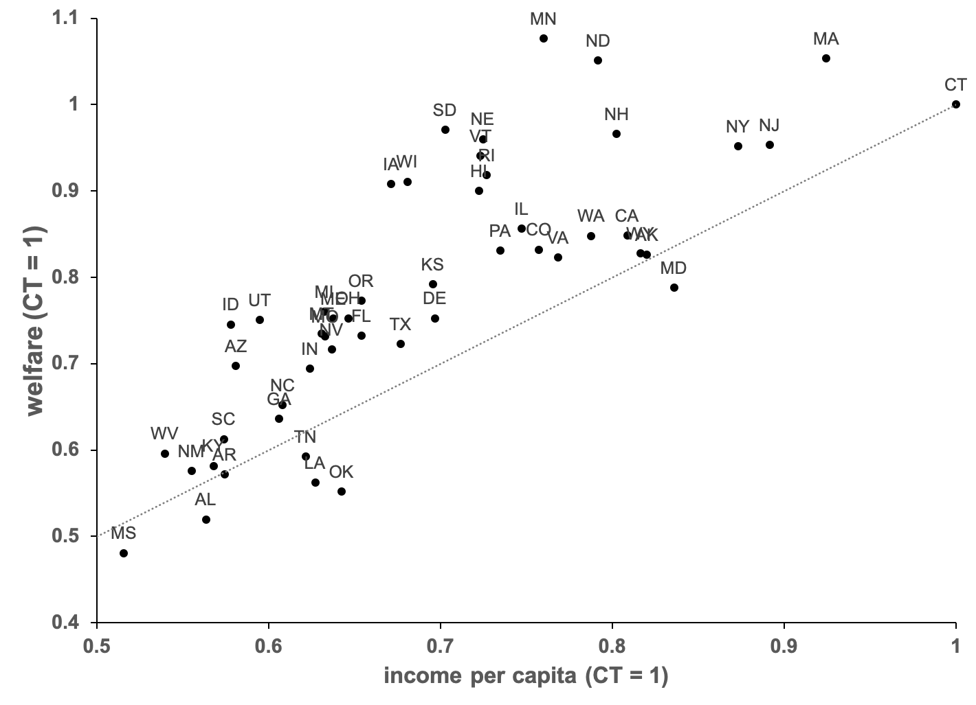
Sources: The welfare level for every state is derived through the authors' calculations and normalized by the corresponding value in Connecticut. In particular, we quantify the welfare differences across states by computing how much spending must change in all ages in the state with the highest personal income per capita, Connecticut, to make an unborn agent under the veil of ignorance indifferent between living her entire life in Connecticut and any other state. The dashed line is a 45 degree line where welfare coincides with income per capita. Real personal income per capita is calculated based on releases of the Bureau of Economic Analysis: "SAINC1 Personal Income Summary: Personal Income, Population, Per Capita Personal Income," 2012-2017 Personal Income Data, U.S. Bureau of Economic Analysis, Web. October 2019; "Personal Consumption Expenditures" from: "Table 2.3.4. Price Indexes for Personal Consumption Expenditures by Major Type of Product," 2012-2017, with 2012 as base year, U.S. Bureau of Economic Analysis, Web. October 2019. Values for income per capita refer to five-year averages between 2012 and 2017.
This shows that richer states tend to have higher living standards than poorer states. While welfare and per capita income are positively correlated, deviations between the two measures are often large. For instance, states such as Iowa, Minnesota, and South Dakota have 35.3–41.6 percent higher welfare than per capita income. In contrast, states such as Alabama, Louisiana, and Oklahoma have 7.8–14.1 percent lower welfare than per capita income. A comparison across all states shows that states tend to have higher welfare than per capita income, with a population-weighted average deviation of 10.1 percent across states.
We also find that inequality in welfare, as measured by the dispersion in welfare levels across states, exceeds the corresponding inequality in per capita income levels in the United States. In particular, while income per capita is 48.4 percent higher in the state with the highest income, Connecticut, than in the state with the lowest income, Mississippi, welfare is 55.3 percent higher in the state with the highest welfare, Minnesota, than in the state with the lowest welfare, Mississippi.
We then use the model to study the determinants of the welfare differences across the United States. Table 1 reports each state's welfare and income levels, all indexed to Connecticut (=100), as well as the decomposition of the determinants of welfare, reported in log points. In particular, we decompose the welfare differences into differences in life expectancy, college attainment, average spending, inequality, consumption-good prices, and housing prices.
Table 1: Comparing welfare across the United States
| Decomposition | ||||||||
|---|---|---|---|---|---|---|---|---|
| State | Welfare | Income | Life expectancy | College attainment | Consumption | Inequality | Consumption prices | Housing prices |
| MN | 107.6 | 76.0 | 0.028 [80.7] |
-0.005 [44.3] |
-0.118 [35.5] |
0.062 [0.13] |
0.066 [0.98] |
0.041 [0.95] |
| MA | 105.4 | 92.4 | -0.049 [80.2] |
0.051 [50.9] |
0.021 [40.7] |
0.019 [0.17] |
0.024 [1.03] |
-0.013 [1.23] |
| ND | 105.1 | 79.2 | -0.038 [79.5] |
-0.105 [32.8] |
-0.031 [38.7] |
0.047 [0.15] |
0.106 [0.93] |
0.073 [0.83] |
| CT | 100.0 | 100.0 | 0.000 [80.6] |
0.000 [44.9] |
0.000 [39.9] |
0.000 [0.19] |
0.000 [1.06] |
0.000 [1.15] |
| SD | 97.1 | 70.3 | -0.064 [79.0] |
-0.101 [33.2] |
-0.156 [34.2] |
0.062 [0.13] |
0.116 [0.92] |
0.113 [0.68] |
| NH | 96.6 | 80.2 | -0.082 [79.4] |
-0.039 [40.2] |
-0.020 [39.1] |
0.079 [0.11] |
0.033 [1.02] |
-0.006 [1.19] |
| NE | 96.0 | 72.5 | -0.054 [79.3] |
-0.044 [39.7] |
-0.210 [32.4] |
0.070 [0.12] |
0.106 [0.93] |
0.091 [0.76] |
| NJ | 95.3 | 89.2 | -0.031 [80.1] |
0.007 [45.7] |
-0.010 [39.5] |
0.022 [0.17] |
-0.005 [1.07] |
-0.031 [1.33] |
| NY | 95.2 | 87.3 | 0.024 [80.6] |
0.014 [46.5] |
-0.002 [39.7] |
-0.030 [0.22] |
-0.024 [1.10] |
-0.032 [1.34] |
| VT | 94.1 | 72.3 | -0.07 [79.6] |
-0.042 [39.9] |
-0.072 [37.2] |
0.065 [0.13] |
0.057 [0.99] |
0.000 [1.16] |
| RI | 91.8 | 72.7 | -0.052 [79.6] |
-0.016 [43.0] |
-0.128 [35.1] |
0.025 [0.17] |
0.053 [0.99] |
0.032 [0.99] |
| WI | 91.1 | 68.1 | -0.034 [79.4] |
-0.092 [34.1] |
-0.189 [33.0] |
0.063 [0.13] |
0.094 [0.94] |
0.065 [0.86] |
| IA | 90.8 | 67.1 | -0.036 [79.3] |
-0.063 [37.4] |
-0.263 [30.7] |
0.066 [0.13] |
0.108 [0.93] |
0.092 [0.75] |
| HI | 90.0 | 72.2 | 0.104 [81.5] |
-0.152 [28.4] |
-0.101 [36.1] |
0.077 [0.12] |
0.035 [1.02] |
-0.069 [1.59] |
| IL | 85.6 | 74.7 | -0.103 [78.9] |
-0.009 [43.8] |
-0.151 [34.3] |
0.019 [0.17] |
0.056 [0.99] |
0.033 [0.99] |
| CA | 84.8 | 80.9 | 0.050 [80.9] |
-0.095 [34.0] |
-0.111 [35.7] |
0.010 [0.18] |
0.035 [1.02] |
-0.054 [1.48] |
| WA | 84.8 | 78.8 | -0.027 [80.0] |
-0.089 [34.3] |
-0.132 [35.0] |
0.055 [0.14] |
0.027 [1.03] |
0.002 [1.15] |
| CO | 83.2 | 75.7 | -0.061 [80.1] |
-0.049 [39.0] |
-0.190 [33.0] |
0.056 [0.14] |
0.060 [0.99] |
0.001 [1.15] |
| PA | 83.1 | 73.5 | -0.138 [78.2] |
-0.035 [40.6] |
-0.143 [34.6] |
0.030 [0.16] |
0.044 [1.01] |
0.057 [0.89] |
| WY | 82.8 | 81.6 | -0.098 [78.4] |
-0.169 [24.6] |
-0.125 [35.2] |
0.081 [0.11] |
0.070 [0.97] |
0.052 [0.91] |
| AK | 82.6 | 82.0 | -0.191 [77.8] |
-0.159 [25.3] |
0.023 [40.9] |
0.100 [0.09] |
0.074 [0.97] |
-0.039 [1.38] |
| VA | 82.3 | 76.8 | -0.107 [79.0] |
-0.049 [38.8] |
-0.135 [34.9] |
0.038 [0.15] |
0.050 [1.00] |
0.008 [1.11] |
| KS | 79.2 | 69.6 | -0.139 [78.4] |
-0.041 [39.8] |
-0.300 [29.6] |
0.053 [0.14] |
0.100 [0.94] |
0.093 [0.75] |
| MD | 78.8 | 83.6 | -0.141 [78.9] |
-0.039 [40.2] |
-0.122 [35.3] |
0.063 [0.13] |
0.015 [1.04] |
-0.015 [1.24] |
| OR | 77.3 | 65.4 | -0.060 [79.4] |
-0.122 [30.2] |
-0.212 [32.3] |
0.047 [0.15] |
0.065 [0.98] |
0.025 [1.03] |
| MI | 76.0 | 63.2 | -0.160 [77.8] |
-0.081 [34.8] |
-0.225 [31.8] |
0.037 [0.16] |
0.080 [0.96] |
0.076 [0.81] |
| DE | 75.2 | 69.7 | -0.133 [78.4] |
-0.111 [31.3] |
-0.167 [33.8] |
0.051 [0.14] |
0.041 [1.01] |
0.035 [0.98] |
| OH | 75.2 | 64.6 | -0.217 [77.0] |
-0.111 [30.8] |
-0.199 [32.7] |
0.037 [0.16] |
0.107 [0.93] |
0.099 [0.73] |
| ME | 75.2 | 63.8 | -0.115 [78.5] |
-0.162 [24.9] |
-0.158 [34.1] |
0.055 [0.14] |
0.053 [0.99] |
0.043 [0.95] |
| UT | 75.1 | 59.5 | -0.052 [79.5] |
-0.147 [27.0] |
-0.289 [29.9] |
0.090 [0.10] |
0.064 [0.98] |
0.047 [0.93] |
| ID | 74.5 | 57.8 | -0.052 [79.1] |
-0.125 [29.8] |
-0.338 [28.5] |
0.061 [0.13] |
0.075 [0.97] |
0.085 [0.78] |
| MT | 73.5 | 63.1 | -0.144 [78.3] |
-0.107 [31.7] |
-0.252 [31.0] |
0.051 [0.14] |
0.073 [0.97] |
0.070 [0.83] |
| FL | 73.2 | 65.4 | -0.045 [79.5] |
-0.112 [31.8] |
-0.254 [30.9] |
0.012 [0.18] |
0.068 [0.98] |
0.019 [1.06] |
| MO | 73.2 | 63.3 | -0.219 [77.2] |
-0.107 [31.3] |
-0.120 [30.7] |
0.043 [0.15] |
0.105 [0.93] |
0.096 [0.74] |
| TX | 72.3 | 67.7 | -0.116 [78.5] |
-0.105 [31.9] |
-0.238 [31.4] |
0.019 [0.17] |
0.067 [0.98] |
0.048 [0.93] |
| NV | 71.7 | 63.7 | -0.133 [78.0] |
-0.187 [21.9] |
-0.169 [33.7] |
0.052 [0.14] |
0.063 [0.98] |
0.040 [0.96] |
| AZ | 69.7 | 58.1 | -0.049 [79.4] |
-0.120 [30.7] |
-0.346 [28.2] |
0.037 [0.16] |
0.069 [0.97] |
0.049 [0.92] |
| IN | 69.4 | 62.4 | -0.215 [76.9] |
-0.120 [29.6] |
-0.276 [30.3] |
0.055 [0.14] |
0.098 [0.94] |
0.094 [0.75] |
| NC | 65.2 | 60.8 | -0.162 [77.7] |
-0.090 [33.6] |
-0.374 [27.4] |
0.022 [0.17] |
0.094 [0.94] |
0.081 [0.79] |
| GA | 63.6 | 60.6 | -0.208 [77.3] |
-0.098 [32.3] |
-0.327 [28.8] |
0.017 [0.18] |
0.086 [0.95] |
0.078 [0.81] |
| SC | 61.3 | 57.4 | -0.244 [76.7] |
-0.092 [32.9] |
-0.368 [27.6] |
0.029 [0.16] |
0.096 [0.94] |
0.089 [0.76] |
| WV | 59.6 | 54.0 | -0.351 [75.0] |
-0.108 [30.4] |
-0.331 [28.6] |
0.033 [0.16] |
0.111 [0.92] |
0.129 [0.64] |
| TN | 59.2 | 62.2 | -0.304 [75.9] |
-0.083 [33.7] |
-0.344 [28.3] |
0.017 [0.18] |
0.098 [0.94] |
0.093 [0.75] |
| KY | 58.2 | 56.8 | -0.320 [75.4] |
-0.121 [28.7] |
-0.343 [28.3] |
0.017 [0.18] |
0.111 [0.92] |
0.114 [0.68] |
| NM | 57.6 | 55.5 | -0.183 [77.7] |
-0.207 [19.1] |
-0.338 [28.5] |
0.030 [0.16] |
0.071 [0.97] |
0.075 [0.82] |
| AR | 57.2 | 57.5 | -0.304 [75.6] |
-0.141 [26.1] |
-0.384 [27.2] |
0.024 [0.17] |
0.116 [0.92] |
0.130 [0.63] |
| LA | 56.2 | 62.7 | -0.324 [75.6] |
-0.115 [29.5] |
-0.320 [28.9] |
-0.002 [0.20] |
0.096 [0.94] |
0.089 [0.76] |
| OK | 55.2 | 64.2 | -0.326 [75.5] |
-0.156 [23.9] |
-0.361 [27.8] |
0.038 [0.16] |
0.104 [0.93] |
0.106 [0.71] |
| AL | 51.9 | 56.3 | -0.356 [75.2] |
-0.166 [22.2] |
-0.394 [26.9] |
0.018 [0.17] |
0.112 [0.92] |
0.130 [0.63] |
| MS | 48.1 | 51.6 | -0.384 [74.6] |
-0.178 [20.3] |
-0.437 [25.8] |
0.017 [0.18] |
0.121 [0.91] |
0.129 [0.64] |
Sources: Authors' calculations. Column 2 reports how much spending must change in all ages in Connecticut to make an unborn agent under the veil of ignorance indifferent between living her entire life in Connecticut and any other state. Column 3 reports each state's income per capita relative to Connecticut. The welfare decomposition in columns 4–9, reported in log points, decomposes the welfare differences into differences in six parts: life expectancy; college attainment; average spending; inequality; consumption-good prices; and housing prices. Values in square brackets report state-specific life expectancy at birth, college attainment of 25–29 year-olds, demographic-adjusted per capita consumption of non-durables and services, variance of spending, price of consumption goods relative to the average price level in the US, and price of housing relative to the average price level in the US.
We find that lower life expectancy and lower average spending in low-income states account for most of the lower welfare in these states compared with high-incomes states. Lower college attainment further reduces welfare in low-income states. Low-income states, however, generally benefit from lower cost of living as reflected in lower prices of consumption goods and lower housing prices. Therefore, failure to account for the heterogeneity in cost of living would lead one to overestimate the dispersion in welfare between high- and low-income states.
To better understand these results, let us compare living standards in Hawaii and Connecticut. The welfare level in Hawaii is equal to 90.0, which means that living standards (measured as expected lifetime utility) are 10.0 percent lower in Hawaii than in Connecticut. That is, spending in Connecticut would have to decrease 10.0 percent for Janet to be completely indifferent between living her entire life in Connecticut and in Hawaii.
The decomposition tells us why living standards are higher in Connecticut than in Hawaii. The values in brackets report data statistics for each variable in the decomposition. From those, it is easy to see where Hawaii wins: It has higher life expectancy (81.5 vs. 80.6), lower inequality (0.12 vs. 0.19), and lower consumption prices (1.02 vs. 1.06); and where Hawaii loses: It has lower college attainment (28.4 vs. 44.9), lower spending (36.1 vs. 39.9), and higher housing prices (1.59 vs. 1.15). As an example of the actual decomposition, the log points attached to housing prices in Hawaii is -0.069, which means that the higher housing prices in Hawaii reduce welfare in Hawaii by 6.9 log points relative to Connecticut. Because of logarithmic properties, this is approximately equal to saying that higher housing prices reduce welfare in Hawaii 6.9 percent relative to Connecticut. Similarly, higher life expectancy in Hawaii increases welfare in Hawaii 10.4 log points relative to Connecticut. This means that higher life expectancy in Hawaii increases welfare in Hawaii approximately 10.4 percent relative to Connecticut. Intuitively, since the overall welfare is lower in Hawaii than in Connecticut, it must mean that the negative factors are negative enough to cancel out the effect of the positive ones. In this case, living standards are higher in Connecticut than in Hawaii because of higher college attainment, lower housing prices, and higher spending in Connecticut.
Quantitative Findings – Welfare Comparison Over Time
Finally, we use the model to quantify each state's welfare growth rate between 1999 and 2015 to examine how each state's living standards have evolved over time. This is motivated by the fact that changes in life expectancy, college attainment, spending, inequality, consumption-good prices, and housing prices have varied considerably across states. The results are reported in Table 2.
Table 2: Comparing welfare across time: Annual growth in welfare
| Decomposition | ||||||||
|---|---|---|---|---|---|---|---|---|
| State | Growth in welfare | Growth in income | Life expectancy | College attainment | Consumption | Inequality | Consumption prices | Housing prices |
| ND | 3.76 | 3.21 | 0.89 [77.4, 79.5] |
0.18 [29.0, 32.8] |
2.95 [22.8, 38.7] |
-0.03 [0.14, 0.15] |
-0.04 [0.92, 0.93] |
-0.18 [0.72, 0.83] |
| NY | 3.66 | 1.67 | 1.45 [77.4, 80.6] |
0.62 [33.0, 46.5] |
1.65 [28.9, 39.7] |
-0.03 [0.22, 0.22] |
-0.02 [1.09, 1.10] |
-0.01 [1.33, 1.34] |
| SD | 3.22 | 2.14 | 0.84 [77.2, 79.0] |
0.23 [28.3, 33.2] |
2.26 [22.5, 34.2] |
0.02 [0.13, 0.13] |
-0.06 [0.91, 0.92] |
-0.06 [0.65, 0.68] |
| NV | 2.99 | 0.39 | 1.25 [75.0, 78.0] |
0.27 [15.8, 21.9] |
1.38 [25.4, 33.7] |
-0.06 [0.13, 0.14] |
-0.06 [0.97, 0.98] |
0.22 [1.13, 0.96] |
| RI | 2.99 | 1.51 | 0.82 [77.6, 79.6] |
0.67 [28.3, 43.0] |
1.58 [25.7, 35.1] |
-0.10 [0.15, 0.17] |
-0.06 [0.98, 0.99] |
0.08 [1.05, 0.99] |
| MD | 2.95 | 1.49 | 1.07 [76.2, 78.9] |
0.39 [31.4, 40.2] |
1.45 [26.5, 35.3] |
-0.02 [0.13, 0.13] |
0.06 [1.06, 1.04] |
0.01 [1.25, 1.24] |
| CT | 2.87 | 1.45 | 1.04 [78.1, 80.6] |
0.60 [31.9, 44.9] |
1.16 [31.3, 39.9] |
-0.03 [0.19, 0.19] |
0.04 [1.07, 1.06] |
0.06 [1.20, 1.15] |
| CA | 2.87 | 1.78 | 1.33 [77.7, 80.9] |
0.32 [27.0, 34.0] |
1.40 [26.9, 35.7] |
-0.08 [0.17, 0.18] |
-0.14 [0.99, 1.02] |
0.05 [1.53, 1.48] |
| NJ | 2.81 | 1.31 | 1.08 [77.6, 80.1] |
0.46 [35.7, 45.7] |
1.36 [30.0, 39.5] |
-0.06 [0.16, 0.17] |
-0.09 [1.05, 1.07] |
0.06 [1.40, 1.33] |
| VA | 2.78 | 1.48 | 1.05 [76.7, 79.0] |
-0.04 [39.8, 38.8] |
1.73 [25.0, 34.9] |
0.01 [0.16, 0.15] |
0.02 [1.00, 1.00] |
0.02 [1.13, 1.11] |
| PA | 2.77 | 1.62 | 0.87 [76.3, 78.2] |
0.40 [31.6, 40.6] |
1.51 [25.7, 34.6] |
-0.01 [0.16, 0.16] |
0.01 [1.01, 1.01] |
0.00 [0.88, 0.89] |
| NE | 2.75 | 1.78 | 0.77 [77.5, 79.3] |
0.45 [29.8, 39.7] |
1.54 [23.9, 32.4] |
0.01 [0.13, 0.12] |
-0.02 [0.93, 0.93] |
0.00 [0.76, 0.76] |
| WY | 2.69 | 2.54 | 0.38 [77.4, 78.4] |
0.24 [19.2, 24.6] |
2.01 [24.1, 35.2] |
0.09 [0.13, 0.11] |
0.03 [0.98, 0.97] |
-0.06 [0.87, 0.91] |
| IL | 2.67 | 1.17 | 0.95 [76.8, 78.9] |
0.45 [33.7, 43.8] |
1.20 [26.8, 34.3] |
-0.04 [0.17, 0.17] |
0.08 [1.01, 0.99] |
0.02 [1.01, 0.99] |
| LA | 2.65 | 1.98 | 0.78 [73.8, 75.6] |
0.34 [21.4, 29.5] |
1.55 [21.3, 28.9] |
-0.05 [0.19, 0.2] |
0.04 [0.95, 0.94] |
-0.01 [0.76, 0.76] |
| DE | 2.55 | 0.67 | 1.07 [76.0, 78.4] |
0.13 [28.5, 31.3] |
1.27 [26.0, 33.8] |
-0.06 [0.13, 0.14] |
0.12 [1.04, 1.01] |
0.02 [1.00, 0.98] |
| HI | 2.55 | 1.64 | 0.87 [79.2, 81.5] |
0.17 [24.9, 28.4] |
1.60 [26.4, 36.1] |
0.05 [0.12, 0.12] |
-0.17 [0.98, 1.02] |
0.04 [1.64, 1.59] |
| MA | 2.55 | 1.74 | 0.96 [77.8, 80.2] |
0.34 [43.4, 50.9] |
1.25 [31.6, 40.7] |
-0.03 [0.17, 0.17] |
0.02 [1.03, 1.03] |
0.02 [1.24, 1.23] |
| MT | 2.53 | 2.32 | 0.36 [77.1, 78.3] |
0.36 [23.6, 31.7] |
1.87 [21.7, 31.0] |
-0.04 [0.14, 0.14] |
0.03 [0.98, 0.97] |
-0.06 [0.80, 0.83] |
| TX | 2.52 | 1.58 | 0.96 [76.2, 78.5] |
0.36 [23.8, 31.9] |
1.19 [24.5, 31.4] |
0.04 [0.18, 0.17] |
0.04 [0.98, 0.98] |
-0.06 [0.88, 0.93] |
| AK | 2.51 | 1.93 | 0.45 [76.4, 77.8] |
0.32 [18.1, 25.3] |
1.63 [29.7, 40.9] |
0.03 [0.10, 0.09] |
0.11 [0.99, 0.97] |
-0.03 [1.35, 1.38] |
| SC | 2.49 | 1.23 | 0.75 [74.9, 76.7] |
0.54 [20.3, 32.9] |
1.15 [21.7, 27.6] |
0.01 [0.17, 0.16] |
0.05 [0.95, 0.94] |
0.00 [0.76, 0.76] |
| MN | 2.43 | 1.46 | 0.95 [78.7, 80.7] |
0.37 [36.5, 44.3] |
1.13 [28.0, 35.5] |
-0.01 [0.13, 0.13] |
0.01 [0.98, 0.98] |
-0.01 [0.95, 0.95] |
| WI | 2.40 | 1.25 | 0.73 [77.8, 79.4] |
0.30 [27.5, 34.1] |
1.41 [24.9, 33.0] |
-0.05 [0.12, 0.13] |
-0.03 [0.94, 0.94] |
0.04 [0.88, 0.86] |
| TN | 2.39 | 1.25 | 0.90 [73.8, 75.9] |
0.51 [21.7, 33.7] |
0.95 [22.9, 28.3] |
0.03 [0.18, 0.18] |
0.03 [0.94, 0.94] |
-0.02 [0.74, 0.75] |
| VT | 2.38 | 1.84 | 0.63 [77.9, 79.6] |
0.24 [34.5, 39.9] |
1.69 [26.8, 37.2] |
-0.05 [0.12, 0.13] |
-0.07 [0.98, 0.99] |
-0.05 [1.11, 1.16] |
| NC | 2.38 | 0.99 | 1.08 [75.4, 77.7] |
0.26 [27.7, 33.6] |
1.05 [21.9, 27.4] |
-0.03 [0.17, 0.17] |
0.03 [0.95, 0.94] |
-0.01 [0.79, 0.79] |
| FL | 2.38 | 1.06 | 1.01 [77.0, 79.5] |
0.33 [24.5, 31.8] |
1.05 [24.7, 30.9] |
-0.03 [0.18, 0.18] |
-0.05 [0.97, 0.98] |
0.06 [1.10, 1.06] |
| NH | 2.37 | 1.41 | 0.35 [78.2, 79.4] |
0.60 [27.0, 40.2] |
1.43 [29.4, 39.1] |
-0.05 [0.11, 0.11] |
-0.01 [1.02, 1.02] |
0.06 [1.24, 1.19] |
| AZ | 2.34 | 1.02 | 1.05 [76.8, 79.4] |
0.45 [20.7, 30.7] |
0.65 [24.0, 28.2] |
-0.04 [0.15, 0.16] |
0.12 [1.00, 0.97] |
0.11 [0.99, 0.92] |
| WV | 2.29 | 1.52 | 0.07 [74.8, 75.0] |
0.36 [22.0, 30.4] |
1.91 [19.9, 28.6] |
-0.01 [0.16, 0.16] |
0.00 [0.92, 0.92] |
-0.05 [0.61, 0.64] |
| WA | 2.22 | 1.61 | 0.80 [77.9, 80.0] |
0.28 [28.2, 34.3] |
1.26 [27.0, 35.0] |
0.00 [0.14, 0.14] |
-0.08 [1.01, 1.03] |
-0.04 [1.12, 1.15] |
| OR | 2.15 | 1.25 | 0.82 [77.3, 79.4] |
0.22 [25.3, 30.2] |
1.19 [25.2, 32.3] |
-0.05 [0.14, 0.15] |
0.03 [0.98, 0.98] |
-0.06 [0.99, 1.03] |
| ID | 2.15 | 1.29 | 0.33 [78.2, 79.1] |
0.35 [22.1, 29.8] |
1.45 [21.3, 28.5] |
-0.08 [0.12, 0.13] |
0.05 [0.98, 0.97] |
0.05 [0.81, 0.78] |
| AR | 2.07 | 1.76 | 0.17 [75.1, 75.6] |
0.35 [17.9, 26.1] |
1.57 [19.9, 27.2] |
-0.01 [0.17, 0.17] |
0.00 [0.92, 0.92] |
-0.02 [0.62, 0.63] |
| IA | 2.07 | 1.63 | 0.47 [78.4, 79.3] |
0.23 [32.5, 37.4] |
1.49 [22.8, 30.7] |
-0.03 [0.12, 0.13] |
-0.05 [0.92, 0.93] |
-0.04 [0.73, 0.75] |
| IN | 2.02 | 1.05 | 0.36 [75.9, 76.9] |
0.45 [19.3, 29.6] |
1.17 [23.7, 30.3] |
-0.04 [0.13, 0.14] |
0.03 [0.95, 0.94] |
0.04 [0.77, 0.75] |
| MI | 2.01 | 0.68 | 0.64 [76.4, 77.8] |
0.36 [26.7, 34.8] |
0.94 [25.9, 31.8] |
-0.05 [0.15, 0.16] |
0.07 [0.97, 0.96] |
0.05 [0.85, 0.81] |
| OH | 2.00 | 1.11 | 0.35 [76.2, 77.0] |
0.20 [26.3, 30.8] |
1.45 [24.5, 32.7] |
-0.04 [0.15, 0.16] |
0.01 [0.93, 0.93] |
0.04 [0.75, 0.73] |
| MS | 1.99 | 1.39 | 0.35 [73.8, 74.6] |
-0.07 [21.9, 20.3] |
1.66 [18.6, 25.8] |
0.07 [0.19, 0.18] |
0.01 [0.91, 0.91] |
-0.02 [0.63, 0.64] |
| GA | 1.94 | 0.73 | 1.05 [74.8, 77.3] |
0.01 [31.9, 32.3] |
0.87 [23.6, 28.8] |
-0.04 [0.17, 0.18] |
0.01 [0.96, 0.95] |
0.03 [0.82, 0.81] |
| UT | 1.93 | 1.64 | 0.59 [77.9, 79.5] |
0.04 [26.1, 27.0] |
1.32 [22.8, 29.9] |
-0.04 [0.10, 0.10] |
-0.01 [0.98, 0.98] |
0.02 [0.95, 0.93] |
| OK | 1.84 | 2.18 | 0.00 [75.4, 75.5] |
0.05 [22.7, 23.9] |
1.76 [19.8, 27.8] |
0.06 [0.17, 0.16] |
0.02 [0.94, 0.93] |
-0.05 [0.68, 0.71] |
| KS | 1.83 | 1.64 | 0.31 [77.7, 78.4] |
0.22 [35.0, 39.8] |
1.37 [22.4, 29.6] |
-0.01 [0.14, 0.14] |
-0.06 [0.93, 0.94] |
0.00 [0.75, 0.75] |
| MO | 1.80 | 1.15 | 0.89 [75.3, 77.2] |
-0.13 [34.3, 31.3] |
1.15 [24.9, 31.7] |
0.00 [0.15, 0.15] |
-0.12 [0.91, 0.93] |
0.01 [0.75, 0.74] |
| CO | 1.63 | 1.20 | 0.94 [77.7, 80.1] |
-0.08 [40.8, 39.0] |
0.80 [27.5, 33.0] |
0.06 [0.15, 0.14] |
0.03 [0.99, 0.99] |
-0.11 [1.06, 1.15] |
| KY | 1.63 | 1.26 | 0.08 [75.2, 75.4] |
0.25 [22.8, 28.7] |
1.31 [21.6, 28.3] |
-0.02 [0.17, 0.18] |
0.03 [0.93, 0.92] |
-0.02 [0.67, 0.68] |
| ME | 1.56 | 1.34 | 0.27 [77.4, 78.5] |
0.04 [24.0, 24.9] |
1.33 [25.9, 34.1] |
-0.03 [0.13, 0.14] |
-0.05 [0.98, 0.99] |
-0.01 [0.94, 0.95] |
| AL | 1.43 | 1.24 | 0.29 [74.4, 75.2] |
-0.08 [24.1, 22.2] |
1.14 [21.1, 26.9] |
0.03 [0.18, 0.17] |
0.04 [0.93, 0.92] |
0.01 [0.64, 0.63] |
| NM | 1.38 | 1.44 | 0.11 [77.0, 77.7] |
-0.10 [21.3, 19.1] |
1.37 [21.5, 28.5] |
-0.03 [0.16, 0.16] |
0.03 [0.98, 0.97] |
0.00 [0.82, 0.82] |
Sources: Authors' calculations. Column 2 reports each state's annual welfare growth rate between 1999 and 2015. Column 3 reports each state's annual per capita income growth rate over this time period. Columns 4–9 decompose each state's welfare growth rate into six parts: changes in life expectancy; changes in college attainment; changes in demographic-adjusted per capita consumption of non-durables and services; changes in the variance of spending; changes in consumption good prices; and changes in housing prices. Values in square brackets report state-specific life expectancy at birth in 1999 and 2015, college attainment of 25–29 year-olds in 1999 and 2015, demographic-adjusted per capita consumption of non-durables and services in 1999 and 2015, variance of spending in 1999 and 2015, price of consumption goods relative to the average price level in the US in 1999 and 2015, and price of housing relative to the average price level in the US in 1999 and 2015. Numbers might not add up due to rounding error.
Column 2 and 3 report the annual growth rate of welfare and per capita income, respectively, between 1999 and 2015. The following columns report the growth rates of each of the six welfare determinants over the same period. While all states experienced positive welfare growth over this period, with a population-weighted average growth rate of 2.49 percent per year across states, deviations are often large. North Dakota had the highest growth in welfare between 1999 and 2015, with an average growth rate of 3.76 percent per year over this period. In contrast, New Mexico had the lowest growth in welfare, with an average growth rate of 1.38 percent per year between 1999 and 2015. To put this in perspective, this is equivalent to saying that, under the current trends, living standards are expected to double every 18.4 years in North Dakota, compared to every 50.2 years in New Mexico.
Moreover, while welfare levels and income levels are highly correlated, we find that welfare growth and per capita income growth are only weakly correlated, with a correlation of 0.38 across states. Deviations between welfare growth rates and per capita income growth rates are often large, with a population-weighted average deviation of 1.09 percentage points across states. For example, income per capita increased by 0.39 percent per year in Nevada between 1999 and 2015. The corresponding increase in welfare, on the other hand, was 2.99 percent per year. Hence, whereas the growth rate in income would suggest that living standards barely increased in Nevada between 1999 and 2015, the growth rate in welfare shows that living standards increased considerably over this period. Similarly, whereas a number of states experienced comparable per capita income growth over this time period, their welfare growth often differed substantially. Using per capita income growth rates as the metric of comparison across states would therefore lead one to incorrectly conclude that several states have experienced similar improvements in living standards. Hence, we argue that the growth rate of per capita income is a poor proxy for improvements in living standards.
We then decompose each state's welfare growth rate into six components: changes in life expectancy, changes in college attainment, changes in average spending, changes in inequality, changes in consumption-good prices, and changes in housing prices. We find that while life expectancy at birth increased in all states between 1999 and 2015, the increase varied considerably across the United States, ranging from 0.1 years in Oklahoma to 3.2 years in New York. A variance decomposition of the dispersion in welfare growth rates shows that variation in life expectancy gains alone accounts for 50.3 percent of the dispersion in welfare growth rates in the United States. We find that variation in college attainment gains and variation in spending growth are the other two key factors and account for, respectively, 13.0 percent and 28.4 percent of the dispersion in welfare growth rates across states.
References
Falcettoni, Elena, and Vegard M. Nygaard (2020). "A Comparison of Living Standards Across the States of America," Finance and Economics Discussion Series 2020-041. Washington: Board of Governors of the Federal Reserve System, https://doi.org/10.17016/FEDS.2020.041.
Jones, C. I., and P. J. Klenow (2016), "Beyond GDP? Welfare across countries and time," American Economic Review, 106: 2426–2457.
Falcettoni, Elena, and Vegard M. Nygaard (2020). "A Comparison of Living Standards Across the States of America," FEDS Notes. Washington: Board of Governors of the Federal Reserve System, May 28, 2020, https://doi.org/10.17016/2380-7172.2545.
Disclaimer: FEDS Notes are articles in which Board staff offer their own views and present analysis on a range of topics in economics and finance. These articles are shorter and less technically oriented than FEDS Working Papers and IFDP papers.