FEDS Notes
October 08, 2020
Fire-Sale Vulnerabilities of Banks: Bank-Specific Risks under Stress and Credit Drawdowns
Chaehee Shin and Maddie White1
Introduction
One channel of shock propagation in the financial system is fire-sale-driven spillover that can take place through asset fire sales and the resulting effect of depressed asset prices on the value of firms' assets. Heightened leverage then induces firms to de-lever, triggering another round of asset fire sales. This note reports new findings on fire-sale vulnerabilities at U.S. bank holding companies (BHCs) and intermediate holding companies (IHCs) of foreign banks, which will be together referred to as firms, or banks. We follow the methodology of Greenwood, Landier, and Thesmar (2015)—one of the most widely used methods to calculate fire-sale spillover in the academic literature—to calculate the fire-sale-driven spillover losses of banks as a share of total system equity. While their baseline model assumes an initial shock of 1 percent decline in the value of all bank assets, this note makes a departure from the uniform shock by allowing for bank-specific initial shocks and discusses the implications.
Specifically, we explore two types of bank-specific shocks. First, we use post-stress results based on the adverse scenario projections of 2013–2019 Dodd-Frank Act Stress Test (DFASTs) for the firms that were subject to DFASTs. Even under a common market distress, realized risks may be different across banks. This approach allows greater alignment with idiosyncratic risks at individual banks. Second, we hypothesize simultaneous drawdowns on bank credit lines, which can take place at the same time market distress is unfolding.2 Banks' exposure to such potential drawdowns is large and varies significantly across banks.
Our results show that bank-specific risks materialized from different types of macroeconomic shocks, and the ways they unfold can significantly affect the magnitude of fire-sale vulnerability by banks and, in some cases, would leave most of the U.S. global systemically important banks (G-SIBs) undercapitalized.3 Specifically, compounding the losses in the adverse scenario in DFAST with fire-sale losses can lead to a minimum post-stress leverage ratio that is 1.78 percentage points lower than under the severely adverse scenario, as of the 2018:Q4 exercise date. If a crisis contemporaneously develops simultaneous draws on bank credit lines, it can increase fire-sale-driven losses as a share of total banking system equity up to 14 percentage points higher, compared with when not assuming draws.
Data and Methodology
Following Greenwood, Landier, and Thesmar (2015), we calculate bank $$i$$'s potential losses from a fire sale at each year-quarter $$t$$ as follows:
$$ (1) \ \ \ \ \ \ \ \ a_{it} \sum_{k\prime} m_{ik\prime t}\ l_{kt} \sum_{i\prime} m_{i\prime k\prime t} \Delta {sell}_{i\prime t} $$
Assume that there is a shock to banks. Reading Equation (1) from the right, $$\Delta{sell}_{it}$$ denotes the dollar amount of assets that bank $$i$$ needs to sell at time $$t$$ in response to a shock. $$m_{ikt} \in [0,1]$$ is $$i$$'s portfolio share in asset class $$k$$ at $$t$$. Therefore, $$\sum_{i\prime} m_{i\prime k\prime t} \Delta {sell}_{i\prime t}$$ for an asset class $$k\prime$$ calculates the total dollar amount of $$k\prime$$ sold by all banks in the sample $$i\prime \in I$$ in response to the shock. Moving to the left of Equation (1), $$l_{kt}$$ measures the price effect on asset class $$k$$ at $$t$$.4 Then, $$ \sum_{k\prime} m_{ik\prime t}\ l_{kt} \sum_{i\prime} m_{i\prime k\prime t} \Delta {sell}_{i\prime t} $$ for bank $$i$$ calculates $$i$$'s total percentage of assets that is lost as a result of price effects coming from fire sales of all $$k\prime \in K$$ assets by all banks $$i\prime \in I$$ in the system. Multiplying the term by $$a_{it}$$, $$i$$'s total assets at $$t$$, expresses the total fire-sale-driven loss in terms of dollar amount.
To obtain an aggregate index of fire-sale vulnerability over time, we take the total fire-sale-driven loss across all banks in our sample (that is, adding up outcomes from equation (1) across all banks) and divide it by their total amount of Tier 1 equity capital, $$\sum_i e_{it}$$, at each point in time:
$$ (2) \ \ \ \ \ \ \ \ \frac{ \sum_i a_{it} \sum_{k\prime} m_{ik\prime t}\ l_{kt} \sum_{i\prime} m_{i\prime k\prime t} \Delta {sell}_{i\prime t} }{ \sum_i e_{it} } $$
We use merger-adjusted FR Y-9C data to obtain most of the variables for our sample banks: total assets, Tier 1 equity capital, and portfolio shares of 17 asset classes.5
Aggregate Fire-Sale Vulnerabilities of DFAST Firms Using Post-Stress Outcomes
The first bank-specific shock that we assume comes from each bank's post-stress drop in Tier 1 equity capital in the past DFASTs. Specifically, we define the amount each bank needs to sell in response to the initial shock as the following:
$$ (3) \ \ \ \ \ \ \ \ \Delta {sell}_{it} = b_{it} \Delta e_{it} $$
where $$\Delta e_{it}$$ is the dollar amount of post-stress drop in Tier 1 equity capital of i at $$t$$ and $$b_{it} = d_{it}/e_{it} $$ is the leverage defined as $$i$$'s debt at $$t$$, $$d_{it}$$, over $$i$$'s Tier 1 equity capital at $$t$$, $$e_{it}$$. We compute debt by $$d_{it} = a_{it} - e_{it}$$. A simple assumption here is that banks always target a constant leverage. Therefore, a shock in equity makes banks deviate from their target leverages, leading banks to sell assets to restore their pre-shock leverages.
We obtain $$\Delta e_{it}$$ from the publicly available 2013-2019 DFAST results for the sample of 28 firms that were subject to any of the 2013–2019 DFASTs and consistently reported FR Y-9C from 2009. For each bank, we first collect the bank's percentage drops in minimum Tier 1 leverage ratio under the supervisory adverse scenario from the starting ratio, based on the seven DFAST results, and take its maximum and minimum. Notice the distinction between the definition of (supervisory) Tier 1 leverage ratio and that of leverage above. While leverage is defined as $$b_{it} = d_{it}/e_{it}$$, Tier 1 leverage ratio is defined as Tier 1 capital over total assets, or $$e_{it}/a_{it}$$, following the terminology of our model. Whenever supervisory leverage is referred to in this note, it should be read as $$e_{it}/a_{it}$$.
The last step in calculating $$\Delta e_{it}$$ involves backing out the drop in equity capital needed to justify the drop in Tier 1 leverage ratio, assuming debt fixed. Figure 1 shows the distributions of the two moments—maximum and minimum percentage drops in supervisory leverage ratio in blue and red, respectively—across banks. We use percentage drops instead of percentage point drops to take into account the different initial leverage ratios across banks. Clearly, banks end up with vastly different levels of supervisory leverage ratio shocks even under the same DFAST scenarios. Some banks fall by more than 30 percentage from their previous leverage ratio while others barely fall, under the maximum shocks. A few banks actually improve their ratio (implied by negative shocks), under the minimum shocks.
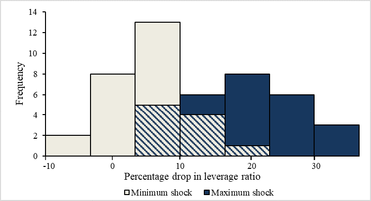
Source: Publicly available DFAST 2019 Supervisory Stress Test Results (June 2019).
Two points are worth mentioning. First, the adverse scenario was chosen because it typically represents a less severe outcome than the severely adverse scenario. In addition, the asset price moves and related economic outcomes in the severely adverse scenario are calibrated under the assumption that liquidity strains and fire sales have occurred. Thus, running fire-sale simulations off of severely adverse scenario results would be double counting. Second, we chose the maximum and minimum of post-stress shocks because the adverse scenario is not always calibrated to be a dampened version of the severely adverse shock. Sometimes it was used to explore important vulnerabilities, such as negative interest rates, that might generate unrepresentative losses. Thus, a time series of losses would not necessarily identify trends in risks and vulnerabilities of these banks.
Figure 2 shows the aggregate fire-sale vulnerabilities of our sample of 28 DFAST firms. Solid lines in black and gray each show results, assuming either the maximum or the minimum shocks from 2013–2019 DFAST post-stress minimum Tier 1 leverage ratios take place for each bank. Based on the maximum shocks, the resulting fire sale will end up affecting as much as 27–56 percent of total system equity. Assuming the minimum shocks significantly lessens the fire-sale-affected system equity to 7–15 percent. Divergence of the two results, or the shaded region between the minimum and maximum effects, highlights the importance of considering the differential effects of macroeconomic shocks on bank-specific outcomes. There are two driving forces behind the wide interval. First, banks substantially vary in terms of magnitude of their post-stress outcomes, as shown in figure 1. Second, banks also differ in terms of other important contributors to aggregate fire sale, such as asset size and leverage. Therefore, aggregate fire-sale vulnerability is not linear in aggregate post-stress outcome.
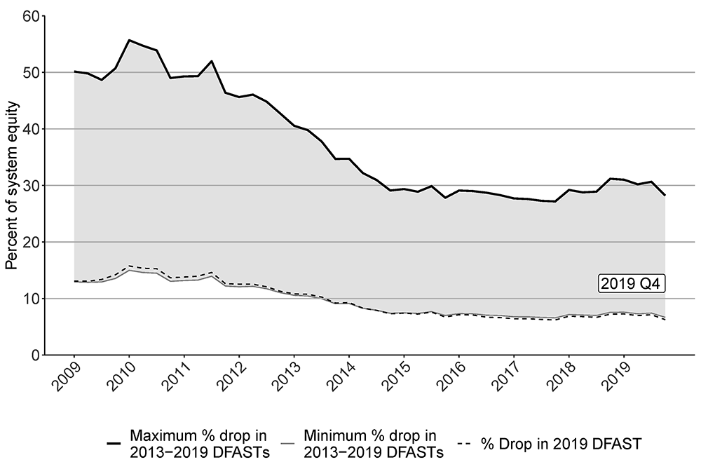
Source: FR Y−9C, Financial Accounts of the United States, publicly available DFAST 2019 Supervisory Stress Test Results (June 2019).
Nevertheless, the range between the maximum and the minimum, which was as wide as 41 percentage points in the years immediately following the Great Financial Crisis, recently narrowed down to about half the magnitude. This narrowing is because banks have built stronger capital base and lowered their leverage so that banks no longer need to sell as many assets in response to a shock. In particular, the dotted line shows results based on the most recent 2019 DFAST shocks, which closely trail those based on the minimum shocks for banks.6
Another way to interpret the magnitude of the aggregate fire-sale vulnerability is to compare the resulting leverage ratios from our model to the post-stress leverage ratios under the severely adverse scenarios of the previous DFASTs. Severely adverse scenarios implicitly assume some propagation mechanism by which shocks spread across the financial system, whereas adverse scenarios generally did not assume that such network and feedback effects were pervasive. Because our model takes initial shocks from the post-stress leverage ratios under the adverse scenarios of the DFASTs and adds the fire-sale effects, the model's outcomes can be compared to those under the severely adverse scenario to see whether the magnitudes look similar.
Table 1: Comparison of Post-Fire-Sale Leverage Ratios to DFAST Post-Stress Leverage Ratios
| Exercise Date: 12/31/2018 | Average across 28 DFAST BHCs (%) |
|
|---|---|---|
| Our model calculation | Post-fire-sale leverage ratio: max shock | 4.94 |
| Post-fire-sale leverage ratio: min shock | 7.97 | |
| Post-fire-sale leverage ratio: 2019 DFAST7 | 7.25 | |
| 2019 severely adverse scenario | Post-stress minimum leverage ratio | 6.72 |
| 2019 adverse scenario | Post-stress minimum leverage ratio | 8.13 |
Source: FR Y-9C, Financial Accounts of the United States, publicly available DFAST 2019 Supervisory Stress Test Results (June 2019).
Table 1 shows the comparison as of 2018:Q4, expressed in terms of averages across all 28 firms in our sample. The effect of a fire sale significantly depends on the initial shock assumption. The average of post-fire-sale leverage ratios under the maximum shock is 4.94 percent, which is 1.78 percentage points lower than the same banks' average post-stress minimum leverage ratio of 6.72 percent under the severely adverse scenario. In this scenario, most U.S. G-SIBs except for two fall below the minimum Tier 1 leverage ratio, 4 percent. Investment banks are among the most severely affected, while regional banks are relatively less affected (not shown); the divergence reflects higher magnitudes of shocks, in general, and a larger asset base of the former. On the other hand, the average post-fire-sale leverage ratios under the minimum shock is 7.97 percent, which lies between the post-stress minimum leverage ratio under the adverse and the severely adverse scenario. The shock based on the most recent 2019 DFAST scenario is close to this rather benign end of the outcome, at 7.25 percent.
Aggregate Fire-Sale Vulnerabilities of Banks with Exposure to Simultaneous Drawdowns on Credit Lines
The second bank-specific shocks that we assume are bank exposures to draws on credit lines. Credit lines are off-balance-sheet items that transition to on balance sheet only when they are drawn. If drawdowns on bank credit lines simultaneously take place in times of widespread market distress, then banks would come under the pressure of selling even more assets—on top of what they were already trying to sell to recover pre-shock leverage—as their post-shock leverage further increases above their target. Note that the resulting fire-sale vulnerability will likely be a conservative estimate because the model hinges on a parsimonious assumption that banks fire-sell in response to a shock due to targeting a constant leverage. If we further incorporate a realistic possibility that short-term funding market may dry up in times of crisis, then banks will need to fire-sell even more assets to raise cash to meet the credit line drawdowns.8
To illustrate the additional effect of simultaneous drawdowns on credit lines, we add to our definition for $$\Delta {sell}_{it}$$, an additional component that represents potential exposure to credit drawdowns as follows:
$$ (4) \ \ \ \ \ \ \ \ \Delta {sell}_{it} = b_{it} \Delta e_{it} + c_{it} $$
where $$c_{it}$$ denotes the dollar amount of total credit drawdowns that bank $$i$$ simultaneously needs to meet at time $$t$$. We obtain an estimate of $$c_{it}$$ from FR Y-14, which reports quarterly stocks of committed lines and their usage in U.S. BHCs, IHCs of foreign banks, and covered savings and loan holding companies (SLHCs) with $100 billion or more assets. For our purpose, we define $$c_{it}$$ as bank $$i$$'s self-reported estimate of exposure at default (EAD) for the unused portion of total committed lines that $$i$$ has extended as of time $$t$$. EAD is the bank's estimate of the potential future exposure when a loan defaults; that is, the amount that the bank estimates that borrower would draw down if it were under stress.
Potential exposures are large in magnitude and vary significantly across banks. Figure 3 shows the distributions of total unused committed lines and EAD of the unused lines as a share of total assets, respectively, across 23 banks in our FR Y-14 – FR Y-9C matched sample as of 2019:Q4. Average share of undrawn amount out of total assets is 18.1 percent and, among that, the average share of EAD reaches 12.9 percent of total assets. Some banks have high exposures in terms of unused credit lines, reaching 34.1 percent of their total assets, while others have close to zero exposure.9 Banks also exhibit a wide spectrum of EAD on undrawn credit lines, with some banks' aggregate amount of exposure at default reaching nearly 24 percent of total assets while some banks' exposure is close to zero.
Figure 3. Unused Credit Lines and Exposure at Default of Unused Credit Lines as a Share of Total Assets, 2019:Q4
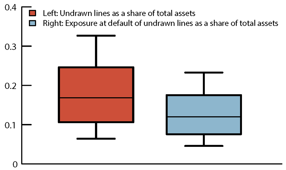
Source: FR Y-9C, Financial Accounts of the United States, FR Y-14. Authors’ calculation.
Figure 4 shows the resulting aggregate fire-sale vulnerabilities of our sample assuming simultaneous drawdowns tantamount to their total EAD on undrawn credit lines, based on the 26 banks in our FR Y-14 – FR Y-9C matched sample. As the benchmark, the dotted line shows the baseline result based on Greenwood, Landier, and Thesmar's (2015) uniform 1 percent asset price shock without assuming any credit drawdowns. The solid line shows the aggregate fire-sale vulnerability when assuming simultaneous credit drawdowns on top of the baseline 1 percent shock to all banks. Although the divergence between the two series has slightly risen over the recent few years, the gap has not widened too much over the period. That is, adding the simultaneous drawdowns on credit lines exposed a range of 11 to 14 percentage points more of system equity to fire-sale vulnerability than the benchmark shock.
Importantly, the potential exposure itself has grown significantly over the same period. The bars indicate the aggregate exposure at default on undrawn credit lines as a share of aggregate total assets. This aggregate share has grown substantially from 8.3 percent to 11.5 percent over the sample period. Together with the minimally affected fire-sale vulnerabilities by potential credit drawdowns, it partly implies that the overall decline in bank leverage since the Great Financial Crisis has played a beneficial role in reducing the effect of credit drawdown on fire sale. On the other hand, it also signifies that, especially after the banks stabilized in terms of post-crisis leverage, the increase in credit drawdown exposure has been less acute at banks that are larger in size, more overlapping in assets with other banks, and/or have a high leverage. Hypothetically, if the credit lines had grown asymmetrically faster at those banks, or even proportionally at all banks, the additional effect of simultaneous credit drawdowns would have followed the rising trend in potential exposure over the same period.
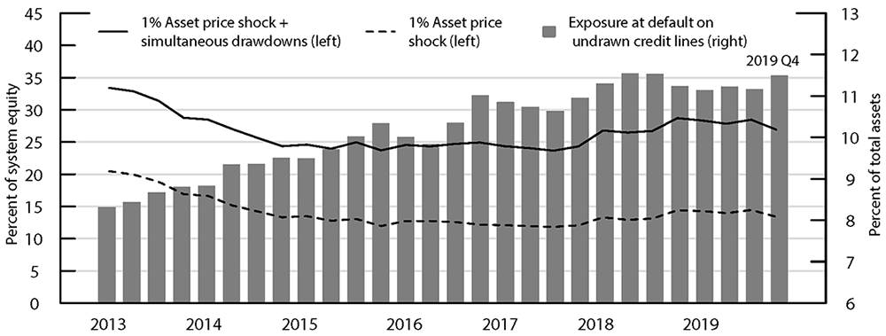
Source: FR Y-9C, Financial Accounts of the United States, FR Y-14. Authors’ calculation.
Conclusion
Banks greatly vary in terms of business model, balance sheet, and capital structure. Different types of recessions lead to bank-specific magnitudes and unfolding of shocks. Combined with heterogeneous leverage, size, and holdings of (illiquid) assets, bank-specific outcomes can result in a wide spectrum of aggregate fire-sale vulnerability. These varying vulnerabilities can sometimes lead to undercapitalization at many U.S. banks, but in other times they can lessen the effect of the fire sale. This approach has the advantage that it can recognize and reflect the heterogeneity embedded in ongoing developments of individual bank risks.
References
Berrospide, Jose M., and Ralf Meisenzahl (2015). "The Real Effects of Credit Line Drawdowns," Finance and Economics Discussion Series 2015-007. Washington: Board of Governors of the Federal Reserve System, February, http://dx.doi.org/10.17016/FEDS.2015.007.
Duarte, Fernando, and Thomas M. Eisenbach (2018). "Fire-Sale Spillovers and Systemic Risk," Staff Report No. 645. New York: Federal Reserve Bank of New York, December.
Greenwood, Robin, Augustin Landier, and David Thesmar (2015). "Vulnerable Banks," Journal of Financial Economics, vol. 115 (March), pp. 471–485.
Ivashina, Victoria, and David Scharfstein (2010). "Loan Syndication and Credit Cycles," American Economic Review, vol. 100 (May), pp. 57–61.
1. We thank William Bassett, Jose Berrospide, Thomas Eisenbach, Erik Heitfield, Elizabeth Klee, Chiara Scotti, and Vladimir Yankov for helpful discussions and comments. The views expressed here are strictly those of the authors and do not necessarily represent the views of the Federal Reserve Board or the Federal Reserve System. Return to text
2. See Ivashina and Scharfstein (2010) and Berrospide and Meisenzahl (2015), among others. Return to text
3. As of 2018:Q4 exercise date. Return to text
4. Following Greenwood, Landier, and Thesmar (2015), we simplify the price effects so that $$l_{kt}=l_t$$ for all $$k$$. We further standardize by anchoring them around 2011 Q3 – for which we assume $$l_{2011Q3} = 10^{-13}$$ – and by defining $$l_t = l_{2011Q3} \times \omega_{2011Q3} / \omega_t$$, where $$\omega_t$$ is the total amount of financial sector assets at $$t$$. $$l_{2011Q3}=10^{-13}$$ translates to a 10 basis point price effect per $10 billion of assets sold in 2011:Q3. We obtain $$\omega_t$$ from the Financial Accounts of the United States and subtract the aggregate value of assets in our sample banks from the total. Return to text
5. Following the classification by Duarte and Eisenbach (2018), we group assets into the following 17 classes: Cash, U.S. Treasuries, Agency Securities, Municipal Securities, Agency MBS, Non-agency MBS, ABS & Other Debt Securities, Equities & Other Securities, Residual Securities, Repo and Fed Funds Loans, Residential Real Estate Loans, Commercial Real Estate Loans, Other Real Estate Loans, C&I Loans, Consumer Loans, Lease Financings, Residual Loans, and Residual Assets. Return to text
6. Some parts of the series based on 2019 shock are slightly lower than the series based on DFAST minimum shocks because sample of banks subject to DFAST changes over time. Return to text
7. This number is based on a smaller set of 12 banks that was subject to 2019 DFAST and consistently reported FR Y-9C over time. Return to text
8. On the other hand, in time of crises, banks may see high deposit inflows arising from flight to safety. If we loosen the model assumption that each bank targets a constant leverage and instead incorporate other types of bank optimization with respect to liquidity requirement, such as Liquidity Coverage Ratio, the deposit inflows might lessen the need to fire-sell assets. Return to text
9. Since FR Y-14 only reports EAD for total amount of credit lines, we estimate EAD for the unused portion of the credit lines in the following two steps. In Step 1, we pool across all banks and times and obtain average shares of the aggregate $EAD out of the aggregate $committed for the whole sample, and for each of the seven borrower types as in the table below. In Step 2, we estimate the new EAD by multiplying the undrawn amount of the $committed by the corresponding average share from Step 1. Return to text
Shin, Chaehee, and Maddie White (2020). "Fire-Sale Vulnerabilities of Banks: Bank-Specific Risks under Stress and Credit Drawdowns," FEDS Notes. Washington: Board of Governors of the Federal Reserve System, October 08, 2020, https://doi.org/10.17016/2380-7172.2589.
Disclaimer: FEDS Notes are articles in which Board staff offer their own views and present analysis on a range of topics in economics and finance. These articles are shorter and less technically oriented than FEDS Working Papers and IFDP papers.