FEDS Notes
April 08, 2022
Anchored or Not: A Short Summary of a Bayesian Approach to the Persistence of Inflation
Highlights
- Inflation was low and stable in the United States during the first two decades of the 21st century and jumped out of its stable range in 2021. Experience in the early 21st century differed from that of the second half of the 20th century, when inflation showed persistent movements.
- This note summarizes how a Bayesian decisionmaker—aware of the persistence of inflation prior to recent decades and of the experience of the last two decades—would update their assessment of inflation dynamics.
- Given a prior for inflation dynamics consistent with 1960-1999 data, a Bayesian decisionmaker would not update their view of inflation persistence a great deal in light of 2000-2019 data unless they placed very low weight on their prior information.
- This finding implies that the elevated inflation of 2021 may continue into 2022, although inflation would be expected to moderate significantly by 2023.
Consumer price inflation in the United States, as measured by the Consumer Price Index, jumped to just above 7 percent in the twelve months ending in December 2021. Inflation in 2021 reached the highest level seen since the early 1980s. The jump in inflation outside of the range experienced over several decades has raised questions regarding the speed with which, or the degree to which, inflation may return to the 2-percent range consistent with the Federal Reserve's inflation objective.
This note summarizes research that asks how a Bayesian decisionmaker endowed with a prior regarding the inflation process consistent with observed U.S. inflation data over the second half of the 20th century would view the current inflation process. Detailed results are available in Kiley (2022).
1. Data and approach
The study analyses inflation in the United States. The analysis focuses on the Consumer Price Index (CPI), produced monthly by the U.S. Bureau of Labor Statistics. The focus of the investigation is the evolution of the persistence of inflation and, to a lesser extent, the slope of the Phillips Curve. To abstract from the volatility induced by fluctuations in food and energy prices, the empirical work uses the CPI excluding food and energy (core CPI), which is available from January 1957 to January 2022. The results are generally similar for the overall CPI, reflecting the correlation between overall and core CPI (e.g., Kiley, 2008a). The results are also similar when the price index considered is the chain-weighted price index for personal consumption expenditures (PCE prices).
The Phillips Curve framework relates inflation to a measure of economic slack. The analysis uses the unemployment rate of the civilian noninstitutional population aged 16 and over (the unemployment rate), produced monthly by the U.S. Bureau of Labor Statistics.
Figure 1 presents the data on inflation and the unemployment rate. The inflation measure presented is the 12-month change in the natural logarithm of the core CPI (upper panel). From 2000 until 2019, inflation was generally low—near 2 percent—and stable. Inflation jumped out of its 2000-2019 range in 2021, reaching about 5-1/2 percent (according to this measure) in December 2021.
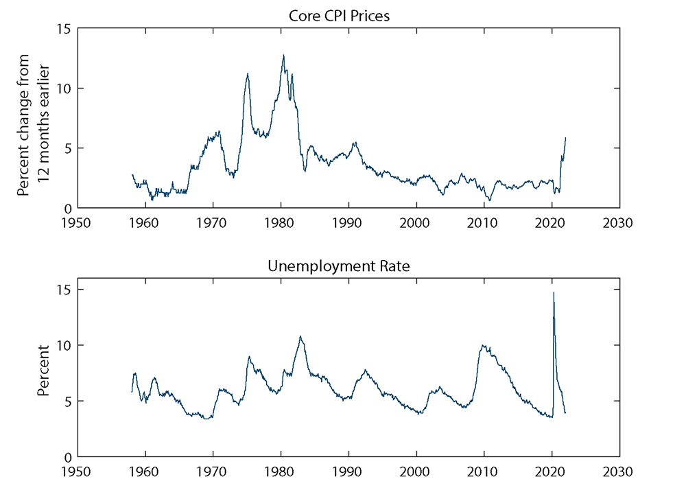
Source: Bureau of Labor Statistics and author’s calculations.
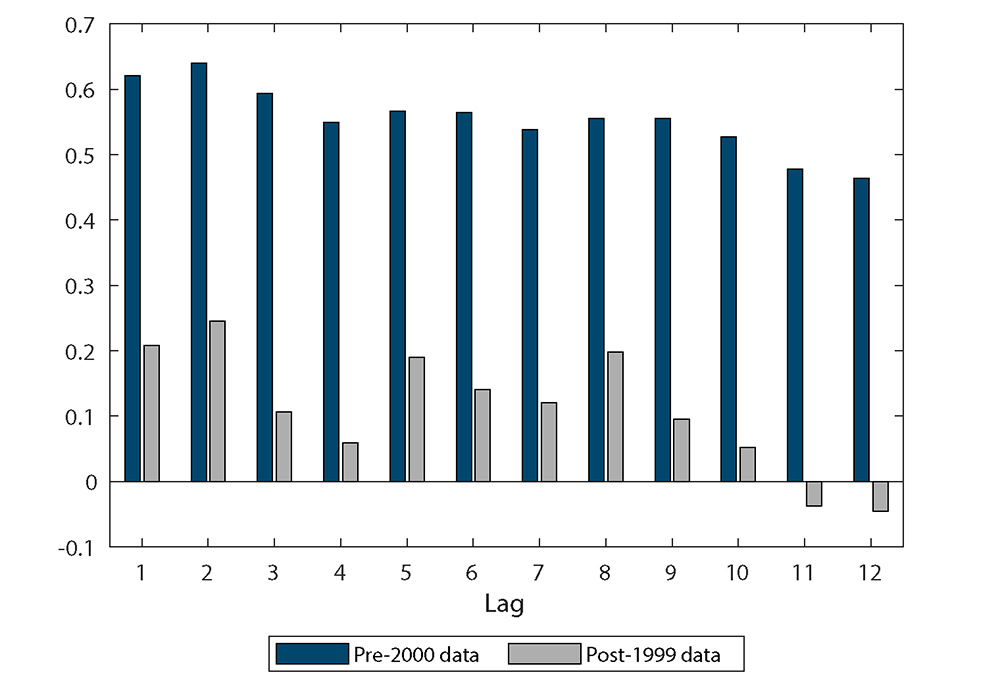
Table 1 presents some summary statistics on inflation and the unemployment rate. Statistics are shown for three sample periods: late 1950s-2019, late 1950s-1999, and 2000-2019. These three sample periods will be referred to as the full sample, the pre-2000 sample, and the post-1999 sample. The years 2020 and 2021 are excluded from the table and the estimation sample, reflecting the unprecedented (and unusual) effects of the COVID-19 pandemic; econometric work will almost surely explore various ways to treat these unusual years in emerging research.2 Two aspects of the summary statistics will prove important in understanding the results. First, inflation was much more volatile in the pre-2000 period than in the post-1999 period, as can be seen in the standard deviations of the series during the periods. Second, inflation was much more persistent in the pre-2000 period than in the post-1999 period, as can be seen in the autocorrelation of the series. The shift in the persistence of inflation is quite notable, as shown in the plot of autocorrelations for lags 1 to 12 (monthly data) in figure 2. Prior to 2000, the correlation of inflation, on a monthly basis, with the level from a year earlier was high, whereas this correlation fell to essentially zero after 1999.
Table 1. Data Summary Statistics
Monthly data
| Observations | Mean (annual rate) | Std. Deviation | Auto- Correlation | |
|---|---|---|---|---|
| Full sample | ||||
| CPI inflation (percent) | 744 | 3.6 | 0.25 | 0.66 |
| Unemployment rate (percent) | - | 6 | 1.6 | 0.99 |
| Pre-2000 sample | ||||
| CPI inflation (percent) | 504 | 4.3 | 0.27 | 0.62 |
| Unemployment rate (percent) | - | 6 | 1.5 | 0.99 |
| Post-1999 sample | ||||
| CPI inflation (percent) | 240 | 2 | 0.08 | 0.21 |
| Unemployment rate (percent) | - | 5.9 | 1.8 | 0.99 |
Note: Full sample: Jan. 1958-Dec. 2019; Pre-2000 sample: Jan. 1958-Dec. 1999; Post-1999 sample: Jan. 2000-Dec. 2019.
Source: Bureau of Labor Statistics and author’s calculations.
Source: Bureau of Labor Statistics and author’s calculations.
2. Empirical Approach
The analysis considers estimates of a Phillips Curve in which inflation ($$\Delta p(t)$$) depends on its own lags and the (lagged) unemployment rate ($$u(t)$$) as in equation (1) (in which a constant term is suppressed):
$$$$ (1) \ \ \ \ \ \ \Delta p(t) = b(1) \sum_{j=1}^N \Delta p(t-j)/N + a \cdot u(t-1) + e(t). $$$$
$$b(1)$$ is the coefficient governing persistence, $$a$$ is the slope of the Phillips curve, and $$e(t)$$ is the residual reflecting "supply" shocks and other unmodeled factors which follows a Normal distribution ($$e(t) \sim N(0,\sigma^2)$$). An anchored Phillips Curve would tend to have small $$b(1)$$, whereas an unanchored Phillips Curve will tend to have large $$b(1)$$, with a value near 1 representing an unanchored accelerationist Phillips Curve. Note that the lag structure in equation 1 is very restrictive, and results were similar for other specifications.
The analysis considers how a Bayesian decisionmaker would use the data from 2000-2019 to update their prior for the inflation process, where the prior is based in data from the late 1950s to 1999. This is a standard statistical problem, and the working paper provides details.3 To consider decreasing levels of conviction in the relevance of the 20th century prior (i.e., looser priors), four values for weights on the pre-2000 information are considered, with the factor $$w$$ governing the weight on the prior relative to the data taking values of 0.5, 0.2, 0.05, or (approximately) 0. (In this weighting scheme, a weight of 0.5 is equal weight on prior and data—one-half weight on each; these weights only partially determine results, which depend on the precision of information in the prior and data as well as the weight.)
Figure 3 presents the prior distributions for the coefficient on the lags of inflation and the slope of the Phillips Curve for these alternative weights. The priors show high values of persistence (a central tendency for the sum on inflation lags near 1) and a notable slope to the Phillips Curve (i.e., a negative slope with a degree of precision in the prior distribution).4
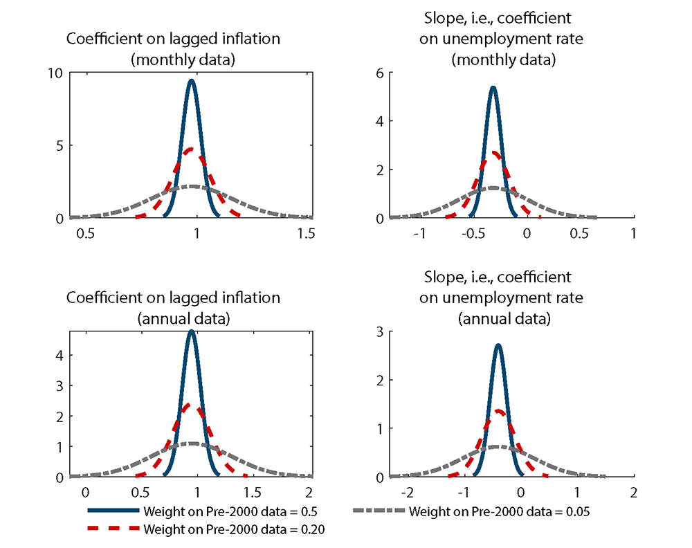
Source: Bureau of Labor Statistics and author’s calculations.
The results for posterior estimates of the Phillips Curve parameters conditional on data from 2000-2019 by the Bayesian decisionmaker are shown in table 2. Two results emerge clearly. First, the degree of persistence in the posterior estimates is high in all cases except those with very little weight on the 20th century information. The coefficient on lagged inflation exceeds 0.9 with equal weights on pre-2000 information and data, exceeds 0.85 when the weight on the pre-2000 information is 0.20, and is near 0.7 when the weight on the pre-2000 information is 0.05; in the limiting case of essentially no weight on the prior, the coefficient on the lags is small at about 0.2 (in line with simple least squares for the 2000-2019 period).
Table 2. Estimation of posterior of parameters
Monthly data (lag length N = 12)
$$$$ \Delta p(t) = b(1) \sum_{j=1}^N \Delta p(t-j) + a \cdot u(t-1) + e(t). $$$$
| Estimates of a Bayesian decisionmaker | Classical least-squares estimates | ||||||
|---|---|---|---|---|---|---|---|
| Weight on pre-2000 information=0.5 | Weight on pre-2000 information=0.2 | Weight on pre-2000 information=0.05 | No weight on pre-2000 information | Full sample | Pre-2000 sample | Post-2000 sample | |
| $$b(1)$$ | 0.92 | 0.86 | 0.66 | 0.17 | 0.95 | 0.97 | 0.17 |
| $$s.e.$$ | 0.03 | 0.05 | 0.1 | 0.16 | 0.03 | 0.04 | 0.16 |
| $$a$$ | -0.07 | -0.04 | -0.06 | -0.13 | -0.19 | -0.32 | -0.13 |
| $$s.e.$$ | 0.03 | 0.03 | 0.03 | 0.04 | 0.05 | 0.07 | 0.04 |
Note: Full sample: Jan. 1958-Dec. 2019 (monthly) and 1959-2019 (annual); Pre-2000 sample: Jan. 1958-Dec. 1999 (monthly) and 1959-1999 (annual); Post-1999 sample: Jan. 2000-Dec. 2019 (monthly) and 2000-2019 (annual).
Source: Bureau of Labor Statistics and author’s calculations.
Second, the slope of the Phillips Curve is consistently smaller in absolute value in the posterior estimates of the parameters—irrespective of the weight on the prior. For example, the slope of the Phillips Curve is less than 1/2 the prior value (the pre-2000 data value from least squares) in the posterior estimates for all weights on the pre-2000 information.
The results are clear—but they are also very intuitive. The posterior estimates combine the prior mean and least-squares estimate for the post-1999 period, with weights given by precision of the information associated with each. Data over the period 2000-2019 provide very little information with which to update prior views on the inflation process, at least with respect to inflation persistence or the "anchoring" of inflation. Inflation was very stable from 2000-2019, which means the data witnessed few substantive deviations from its average or lagged values. Because the data contain few sizable deviations of inflation from its average or lagged values, the data provide little information regarding what would happen if inflation were to deviate sizably from its average or lagged values—an intuitive insight that also follows directly from the mathematics of a Bayesian least-squares regression. The lack of information in the data from 2000-2019 contrast sharply with the precision of the prior view of the role of lagged inflation in the inflation process that is consistent with experience from 1960-1999, when inflation saw sizable swings away from its average value and experience suggests a sizable role for lagged inflation in the Phillips curve. This combination—low information in 2000-2019 data and an informative prior consistent with 1960-1999 experience—implies that the empirical analysis results in substantial inflation persistence unless the prior experience receives very little weight in the Bayesian decisionmaker's calculus.
3. Implications
The implications of the results for inflation in 2022-23 are direct and presented in figure 4 and table 3, which presents forecasts from the monthly estimates assuming that the unemployment rate remains at the level observed in January 2022, 4.0 percent, throughout 2023. A Phillips Curve based on post-1999 data alone would imply a fairly sharp deceleration of inflation in 2022. In contrast, the Bayesian estimates imply that inflation will remain quite high in 2022 in the absence of unexpected shocks.
Table 3. Inflation forecasts for 2022-23
Core CPI inflation, Q4/Q4
| Year | Implied by specifications considered by the Bayesian decisionmaker | Survey of Professional Forecasters | |||
|---|---|---|---|---|---|
| Weight on prior=0.5 | Weight on prior=0.2 | Weight on prior=0.05 | Uninformative prior | February 2022 (median) | |
| 2021 | 5 | 5 | 5 | 5 | 5 |
| 2022 | 5.8 | 5.4 | 4.5 | 3 | 3.6 |
| 2023 | 5.5 | 4.7 | 3.3 | 2.3 | 2.5 |
Note: Author’s calculations based on the estimates for monthly data shown in table 2. The unemployment rate is assumed to remain at its January 2022 value of 4.0 percent.
Source: Bureau of Labor Statistics and author’s calculations.
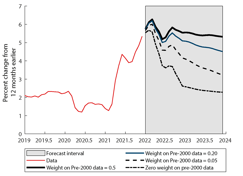
Source: Bureau of Labor Statistics and author’s calculations.
Table 3 also includes the core CPI projection from the February 2022 Survey of Professional Forecasters (Federal Reserve Bank of Philadelphia, 2022). This survey indicates that professional forecasters expected core CPI inflation to drop to 3-1/2 percent in 2022, a result consistent with the view that information on the inflation process prior to the last two decades is irrelevant to the inflation outlook. The results herein suggest a higher degree of persistence is plausible, pointing to potentially higher inflation in 2022.
4. Conclusions
This analysis examined the extent to which the experience from 2000-2019 should lead a Bayesian decisionmaker to update their assessment of inflation dynamics. Given a prior for inflation dynamics consistent with 1960-1999 data, a Bayesian decisionmaker would not update their view of inflation persistence in light of 2000-2019 data unless they placed very low weight on their prior information. In other words, 21st century data contains very little information to dissuade a Bayesian decisionmaker of the view that inflation fluctuations are persistent, or "unanchored".
The idea that data over short sample periods may provide limited information regarding macroeconomic relationships may be relevant for other areas in macroeconomics. For example, Kiley (2020a,b) finds modest information in the data for estimates of the equilibrium real interest rate. These findings suggest macroeconomists may find useful a Bayesian approach that examines the information in the data more thoroughly than is common in empirical macroeconomics.
References
Kiley, Michael T., 2020a. "The Global Equilibrium Real Interest Rate: Concepts, Estimates, and Challenges," Annual Review of Financial Economics, Annual Reviews, vol. 12(1), pages 305-326, December.
Kiley, Michael T., 2020b. "What Can the Data Tell Us about the Equilibrium Real Interest Rate?," International Journal of Central Banking, International Journal of Central Banking, vol. 16(3), pages 181-209, June.
Kiley, Michael T. (2022). "Anchored or Not: How Much Information Does 21st Century Data Contain on Inflation Dynamics?," Finance and Economics Discussion Series 2022-016. Washington: Board of Governors of the Federal Reserve System, https://doi.org/10.17016/FEDS.2022.016.
Lenza, Michele & Giorgio E. Primiceri, 2020. "How to Estimate a VAR after March 2020," NBER Working Papers 27771, National Bureau of Economic Research, Inc.
Primiceri, Giorgio E., 2005. "Time Varying Structural Vector Autoregressions and Monetary Policy," Review of Economic Studies, Oxford University Press, vol. 72(3), pages 821-852.
Schorfheide, Frank & Dongho Song (2021) REAL-TIME FORECASTING WITH A (STANDARD) MIXED-FREQUENCY VAR DURING A PANDEMIC. NBER WORKING PAPER SERIES Working Paper 29535. http://www.nber.org/papers/w29535
1. Federal Reserve Board, Washington DC. Email: [email protected]. Michael Kiley is Deputy Director of the Division of Financial Stability of the Federal Reserve Board. The views expressed herein are those of the author, and do not reflect those of the Federal Reserve Board or its staff. Return to text
2. Lenza and Primiceri (2020) and Schorfheide and Song (2021) highlight the potential sensitivity of macroeconometric estimates to the COVID-19 pandemic period, with the former suggesting some approaches to handling these issues. Return to text
3. Briefly, the vector of coefficients in equation (1) is denoted by $$\Gamma$$. The matrix containing the dependent variable (inflation) will be denoted $$Y$$ ($$T \times 1$$, where $$T$$ is the number of observations), the matrix of right-hand side variables will be denoted $$X$$ ($$T \times N$$), and the matrix of error terms will be denoted $$E$$ ($$T \times 1$$), yielding $$Y=X\Gamma+E$$. The classical approach to inference would estimate $$\Gamma$$ by least squares as $$\Gamma^{LS}=\left(X\prime X\right)^{-1}X^\prime Y$$. The decisionmaker herein follows a Bayesian approach. The decisionmaker is endowed with a prior for $$\Gamma$$ that is given by the Normal distribution with mean $$\widetilde{\Gamma}$$ and variance-covariance matrix $$V$$—i.e., a prior distribution $$\Gamma \sim N(\widetilde{\Gamma},V)$$. Given the prior information, the decisionmaker estimates $$\Gamma$$ by combining their prior information and the data—i.e., the prior distribution and the likelihood function of the data—to form the posterior distribution for $$\Gamma$$ and estimates $$\Gamma$$ to maximize this posterior distribution. The resulting estimate $$\hat{\Gamma}$$ given by $$\hat{\Gamma} = \left(V^{-1}+\sigma^{-2}X^\prime X\right)^{-1}(V^{-1}\widetilde{\Gamma}+\sigma^{-2}X^\prime X\Gamma^{LS})$$. Notice in equation (3) that the Bayesian decisionmaker estimates the parameters as the matrix-weighted average of their prior information and the least-squares estimate, with weights given by the precision of the information in the prior and the data (e.g., by the inverses of the variance-covariance matrices of $$\widetilde{\Gamma}$$ and $$\Gamma^{LS}$$, $$V$$ and $$\sigma^2{(X^\prime X)}^{-1}$$.) The Bayesian decisionmaker can further "weight" their prior by a factor $$w$$, as in $$\hat{\Gamma}\ =\left({wV}^{-1}+\left(1-w\right)\sigma^{-2}X^\prime X\right)^{-1}(wV^{-1}\widetilde{\Gamma}+(1-w)\sigma^{-2}X^\prime X\Gamma^{LS})$$. Mathematically, it is equivalent to considering a less informative prior. Specifically, estimates with a weight of $$w$$ on the prior information are equivalent to estimates with a prior for $$\Gamma$$ with the same mean and a variance-covariance matrix equal to $$\frac{1-w}{w}V$$. For example, a weight on the prior equal to 20 percent ($$w$$=0.2) is equivalent to a prior with a four-times looser variance-covariance matrix $$4V$$. Return to text
4. The estimates use inflation data expressed at annual rates. Return to text
Kiley, Michael T. (2022). "Anchored or Not: A Short Summary of a Bayesian Approach to the Persistence of Inflation," FEDS Notes. Washington: Board of Governors of the Federal Reserve System, April 08, 2022, https://doi.org/10.17016/2380-7172.3049.
Disclaimer: FEDS Notes are articles in which Board staff offer their own views and present analysis on a range of topics in economics and finance. These articles are shorter and less technically oriented than FEDS Working Papers and IFDP papers.