FEDS Notes
August 10, 2020
Are There Competitive Concerns in “Middle Market” Lending?
David Benson and Ken Onishi1
This note analyzes competition and concentration in "middle market" lending using loan level data obtained from large bank holding companies' Y14 reports to the Federal Reserve. The middle market segment is typically considered to be credit for firms larger than small businesses but too small for large-scale commercial lending or syndicated credit. Lender choice and the supply of credit to large and small firms has been studied extensively by academics and policy makers. Yet, much less is known about mid-sized firms' access to capital. Addressing this gap, we study market structure, the geography of borrower-lender proximity, and the persistence of lending relationships from loans supplied to medium-sized businesses in the Y14 data.
Three contributions highlight this work. First, we document patterns in market shares and concentration for an industry which has not received much attention in the literature. Second, we assess what the appropriate geographic market definition is, providing guidance for economic policy and future study of the middle market. Finally, we document middle market borrower inertia in the Y14, providing to our knowledge the first evidence on the extent of lender switching costs for medium-sized businesses.
The economic importance of middle market lending motivates addressing this gap in understanding. Our data contain $549 Billion in credit facilities extended to mid-sized firms, firms with annual revenue between $10 million to $250 million, in the fourth quarter of 2018. Over the same period, middle market credit utilization was relatively high, totaling $355 Billion or about two-thirds of the aggregate credit line.2
Understanding middle market borrowers' access to capital is also important for economic policy. Credit market structure and lender substitutability for mid-sized firms could impact their access to short term lending facilities during a financial crisis, for example. During the COVID19 pandemic, Congress and the Federal Reserve created the Main Street Lending Program to ensure medium-sized businesses had access to needed liquidity.
Additionally, an important open question for antitrust regulators is whether proposed bank mergers should receive more scrutiny for competitive effects on middle market lending. Mergers increase lenders' market power, and hence could increase medium-sized firms' costs of capital. Antitrust authorities routinely scrutinize proposed mergers for their competitive effects on small business lending (Federal Reserve Board, 2020; Department of Justice, 2000), and apparently do not usually scrutinize mergers for competitive effects on large-business lending. Neither the literature nor antitrust regulators have systematic measures of middle market concentration by which to assess a proposed merger's competitive effects, nor is there a consensus geographic market definition to begin such an assessment.
Since there is no consensus geographic market definition, we study market structure at local, regional, and national levels. By examining telescoping geographic market definitions, we are able to provide best and worst case assessments of middle market competition. For each of these market definitions, we describe market concentration using the Herfindahl-Hirschman Index (HHI), the sum of squared market shares within a geographic market. Note that market concentration measured using the Y14 data may overstate or understate actual concentration, since the data do not contain lending activity of non-bank lenders and banks who are not Y14 reporters. In general, we believe that our HHI measure overstates actual market concentration, because non-bank lenders are known to be a significant substitute to traditional banks in the middle market (Chernenko, Erel, and Robert, 2019). We also measure market size, for example documenting the aggregate credit line, and describe the number of middle market borrowers and the number of lenders operating a bank branch in the local market.
We find that at small geographic regions, measured by Federal Reserve banking markets ("Fed markets"), middle market concentration is generally high. There are several monopoly Fed markets, and several markets with neither a middle market borrower or lender. However, at larger geographic regions, measured by states, we find overall low HHIs. No states are monopoly markets, and most states have more than six lenders. Likewise, national market concentration is low. Therefore, whether there are competitive concerns in middle market lending depends on the geographic scope of borrowers' substitution to alternative lenders.
We use a formal test to discern whether a national market, larger regional markets as proxied by states, or smaller local Fed markets are a more appropriate geographic scope for the middle market. The Hypothetical Monopolist test is a common tool used in antitrust practice for this purpose. Our adaptation incorporates the geography of lender substitution observed in the data in order to infer the smallest profit margin necessary and sufficient for a candidate market definition to be profitably controlled by a hypothetical monopolist. The test's economic intuition is that middle market borrowers' willingness to substitute to out-of-market lenders is a key determinant of the profitability of any hypothetical price increase. Our Hypothetical Monopolist test minimal passible margins (MPM) provide a theoretically appropriate metric to gauge the sensibility of narrow versus broader market geographies.
We find that the minimal passible margins for Fed markets are too large to be sensible. In fact, many MPMs are infinite. This suggests that Fed markets are too narrow to appropriately assess competition in the middle market. In comparison, threshold margins for state-based markets are very reasonable. State market MPMs are similar to large banks' return on average assets measured using Call Reports. These results do not necessarily indicate that states are accurate market definitions, but do confirm that middle market geography is broader than Fed markets and have a regional character.
The formal market definition test is necessary because borrowers' proximity to their lenders only provides mixed evidence for the geographic scope of the middle market. The branch location data suggest that medium-sized businesses indeed have a preference for lender proximity. While many mid-sized firms choose an in-market lender, a significant faction are also willing to choose out-of-state or more distant lenders. Furthermore, results from loan-level linear regressions suggest that the borrowing firm's scale, the size of the loan, and expected utilization of the credit line are all negatively correlated with lender proximity.
Therefore, the baseline evidence from borrower-lender proximity does not endorse narrow geographic markets over broader regional markets, or vice versa, and therefore does not confirm or rule out competitive concerns in middle market lending. However, the Hypothetical Monopolist test results do suggest that state-based HHIs more appropriately measure competition for middle market lending. Since state HHIs are generally low, the results paint a picture of relatively healthy competition.
Lenders can obtain market power by means other than market concentration. For example, returns to relationship lending and other information or search frictions can create switching costs. Borrowers with switching costs are less likely to change lenders in response to an interest rate hike or a degradation of quality. We therefore conclude our study with an analysis of borrower inertia. We find that a significant fraction of borrowers switch lenders at the end of their loan term, and that borrowers who switch lenders have similar geographic substitution patterns as were measured using the market cross-sectional data. These results do not suggest that middle market firms have significant switching costs. Instead, middle market firms have substitution patterns which likely facilitates competition among lenders.
Taken together, our findings thus suggest that there are unlikely to be competitive concerns in the provision of middle market financial services. As a matter of economic policy, capital markets for mid-sized firms are likely regional: larger than the borrower's immediate local area but smaller than a national market. Since medium-sized businesses' characteristics and lender choice alternatives vary from region to region, we suggest that monetary authorities account for potential regional variation in the middle market's need for intervention, in particular during a financial crisis. Since state level market concentration is moderate, at most, we also conclude that antitrust authorities should reserve scrutiny to very large bank merger proposals which significantly increase regional market concentration. Such mergers might impact mid-sized firms' access to and costs of capital.
Data & Market Definitions
The Federal Reserve's Y14 quarterly report contains the universe of commercial and industrial (C&I) loans supplied to firms with more than $1 million in sales by stress-tested banks (bank holding companies with more than $100 Billion in assets). In 2018, the largest 30 banking holding companies that operate in the United States filed Y14 reports. Most of our analysis focuses on loans reported in the fourth quarter of 2018. The data include the lender's identity, the loan's committed amount of credit, utilization of this credit line, the duration of the contract, and several characteristics of the borrowing firm including office location and annual sales. In the analysis, we only use C&I loan data that report positive annual sales of borrowers. Lender branch locations data are obtained from the FDIC's June 2018 Summary of Deposits report.
There is no consensus market definition for middle market lending. Antitrust markets have two characteristics, products and geography. The first component involves identifying what types of customers and products should be the focus of the analysis, in this case identifying "middle market" borrowers and loans. The second component involves identifying where consumers' choice alternatives are located, in this case identifying how far away are lenders to which medium-sized businesses are willing to substitute. For a product market definition, we focus on loans made to firms with $10M-$250M in annual sales. This conservative definition is guided by the distribution of firm sizes and loan sizes in the Y14 data, as evidenced later in Figure 1, and is also informed by various by industry and academic publications (Brevoort and Hannan, 2006; Tannenwald, 1994; Elliehausen and Wolken, 1990; Kwast, Starr-McCluer, and Wolken, 1997).3 We use three proxy definitions for the geographic component of the market: Fed banking markets, states, and a national market.
Fed markets are a natural starting point for geographic boundaries of middle market lending. Fed markets are somewhat limited in geographic scope, defined as local economic areas within which representative consumers and small businesses travel for retail banking services. Fed markets often align with MSAs in the vicinity of large urban areas, and often align with counties or collections of smaller municipalities in rural and micropolitan areas.
Fed markets are the starting point antitrust authorities use to measure the competitive effects of bank mergers. Studies suggest that small business lending is a highly local geographic market (FDIC, 2018; Anenberg et al, 2018), potentially smaller even than Fed markets. It is plausible, then, that medium-sized businesses search for lenders in their immediate local area as well. However, due to their size, middle market firms might also have incentives to search more broadly than Fed markets for a credit supplier. Medium-sized businesses have larger balance sheets, a lower external finance premium, and often a wider scope of activity than small businesses. This suggests larger regional geographic markets or perhaps a national market may be more appropriate for middle market lending. We use states as a proxy definition for regional geographic markets.
Market Structure Results
Our market structure analysis begins with the loan-level data. We present the loan-level summary statistics and national aggregates in Table 1.
Table 1: Loan-level Summary Statistics for the Middle Market
| Mean | St. Dev. | 10% | 25% | Median | 75% | 90% | |
|---|---|---|---|---|---|---|---|
| Committed Credit ($M) | 7.1 | 12.9 | 1.1 | 1.6 | 3 | 7.1 | 17 |
| Utilized Credit ($M) | 4.6 | 9.3 | 0 | 0.4 | 1.7 | 4.6 | 11.9 |
| Borrower Sales ($M) | 70.1 | 59.9 | 14.6 | 23.5 | 47.6 | 100.7 | 165.9 |
Aggregates: N Loans 77,070; HHI 737; Committed Credit $549 (B); Utilized Credit $355 (B)
In the fourth quarter of 2018, Y14 filers reported 77,070 outstanding loans to firms with $10M-$250M in annual sales. The average annual sales of middle market borrowers was about $70M, and the firm size standard deviation was about $60M. Committed credit to the middle market totaled $549B, and 65 percent or $355B of total credit was utilized.
The average credit line was $7M and the standard deviation of committed credit was $13M. However, most middle market loans are more modest compared to the average. The median credit limit was only $3M, and the 75th-percentile credit limit was equal to the mean credit limit. The bulk of credit utilization was similarly modest. While average credit utilization was $4.6M, over 10 percent of loans were unutilized and median utilization was $1.7M.
Calculating market concentration using loan-level credit lines provides a national HHI of 737. The national HHI is well below the 1800 threshold that antitrust authorities commonly consider for merger scrutiny (Federal Reserve Board, 2020). In the best case, the middle market is large, economically important, and unconcentrated and fairly competitive.
Is the best case robust to measuring market structure at finer geographic partitions? Table 2 contains summary statistics for Fed markets and states, conditional on the market having at least one borrower and at least one lender.
Table 2: Market Structure Summary Statistics for Fed Markets and States
| Mean | St. Dev. | 10% | 25% | Median | 75% | 90% | |
|---|---|---|---|---|---|---|---|
| Fed Markets | |||||||
| HHI | 5,214 | 3,075 | 1,713 | 2,617 | 4,499 | 8,108 | 10,000 |
| Banks | 5.2 | 5.1 | 1 | 2 | 3 | 7 | 12 |
| Borrowers | 44.1 | 216.7 | 1 | 2 | 5 | 18 | 62 |
| Market Size ($M) | 483 | 2446 | 5 | 13 | 48 | 188 | 643 |
| State Markets | |||||||
| HHI | 1456 | 465 | 886 | 1051 | 1421 | 1759 | 2033 |
| Banks | 21.2 | 5.5 | 13 | 17 | 22 | 26 | 28 |
| Borrowers | 979 | 1,167 | 122 | 197 | 592 | 1,270 | 2,781 |
| Market Size ($M) | 10,766 | 12,835 | 1,208 | 2,173 | 6,329 | 13,413 | 28,783 |
Notes: Calculations based on 1,132 Fed markets and 51 states + DC having at least one middle market borrower. Market size is measured by committed credit, denominated in millions. HHI is the Herfindahl-Hirschman Index, the sum of squared market shares by geographic market.
There are 1,398 Federal Reserve banking markets in 2018, but at least one middle market borrower exists in only 1,132 Fed markets in the Y14 data. We also find that at local geographic markets, middle market concentration is generally high. Roughly 22 percent of Fed markets are monopolies, and the median market only has 3 lenders. Over 75 percent of Fed markets are highly concentrated, defined as an HHI greater than 2500. Consequently, the mean HHI is also high at 5214. Only 132 of the 1,132 Fed markets have HHIs below 1800, the benchmark HHI at which antitrust authorities commonly apply more scrutiny to merger proposals. Thus, if local geographic markets are appropriate for the middle market, the data raise competitive concerns.
However, being unable to measure local market structure because too few borrowers or lenders exist may itself indicate that Fed markets are too narrow to examine middle market lending. Most Fed markets are very small, with few borrowers and even fewer lenders, which naturally results in high market concentration. The median Fed market only has five borrowers, three lenders, and about $48M in credit. Hence, larger geographic markets may be more appropriate for assessing competition.
We proxy for larger geographic regional market definitions using state boundaries. As shown in Table 2, every state has at least one middle market borrower and at least one middle market lender. No state-based markets are monopolies. The average and median state has approximately ten middle market lenders and hundreds of borrowers. At the state level, middle market concentration is overall low. The average state HHI is 1456. The 2500 HHI standard for a highly concentrated market is at least two standard deviations above the mean and median state HHIs. Furthermore, only ten states have HHIs above 1800. Therefore, if broader regional geographic markets are appropriate, the data do not suggest there are competitive concerns in middle market lending.
Preferences for Lender Proximity
The market structure results range from healthy competition in the best case to significant competitive concerns in the worst case, across the telescoping geographic market definitions. Therefore, whether there are competitive concerns in middle market lending depends on the geographic scope of medium-sized businesses' substitution to alternative lenders. To study the scope of substitution, we must measure borrower-lender proximity.
For each geographic market definition, in-market loans and out-of-market loans are identified by whether the lender operates a branch inside the market. The fraction of borrowers choosing an in-market lender reveals that borrowers have preferences for lender proximity. Examining how the in-market lender share changes from smaller/local to larger/regional geographic market definitions provides evidence on the breadth of borrowers' search for lenders.
Table 3: Market-level Variation in the Aggregate In-market Bank Share
| Mean | St. Dev. | 10% | 25% | Median | 75% | 90% | |
|---|---|---|---|---|---|---|---|
| Fed Markets | |||||||
| In-Market Banks | 2 | 2.4 | 0 | 0 | 1 | 3 | 5 |
| Share of In-Market Banks | 36.80% | 35.20% | 0% | 0% | 30.60% | 68.80% | 88.50% |
| State Markets | |||||||
| In-Market Banks | 10.8 | 4.4 | 6 | 7 | 11 | 13 | 17 |
| Share of In-Market Banks | 66.50% | 17.80% | 46.30% | 55.20% | 70.40% | 78.40% | 84.90% |
Notes: Calculations based on 1,132 Fed markets and 51 states + DC having at least one middle market borrower. In-market banks are banks with a branch location inside the geographic market. Market share is measured by committed credit.
Table 3 summarizes the number of in-market banks and their aggregate market share. More than 30 percent of Fed markets, out of 1,132 total markets with at least one middle market borrower, do not have an in-market lender. In the median Fed market, there is only one in-market lender, and that lender typically controls about 30 percent market share. These observations suggest that Fed markets may be too small to use as appropriate geographic boundaries for the middle market, corroborating what was indicated by the inability to measure market structure at the Fed market level for some areas.
At the state market level, the median state has about 30 percent of committed credit supplied by out-of-market banks. The average in-market lender share at the state level is 66.5 percent, nearly double that measured at the Fed market level. With reference to Table 2, notice also that the median state has about the same number of in-market banks and out-of-market banks. Yet, in-market banks have a much larger market share. Taken together, this suggests that borrowers have preferences for lender proximity, especially within-region proximity, but are also willing to search quite broadly for credit.
We explore this preference for proximity further in Figure 1, which shows how lender proximity is associated with borrower and loan characteristics. The upper panel of Figure 1 plots the percentage of committed credit originated from in-market banks versus the borrower's annual sales. The lower panel of Figure 1 plots the percentage of committed credit supplied by in-market banks across loan sizes. In each sub-figure, the solid line measures in-state proximity, and the dashed line measures in-Fed market proximity.
The numbers in Figure 1 are generally higher than the in-market share measures presented in Table 3. In Table 3, the aggregate share of in-market banks was calculated for each geographic market, and the between-market distribution is described. In contrast, Figure 1 measures loan level in-market proximity, which is then averaged over all loans conditional on borrower scale or loan size. Because larger markets tend to have both more loans and more in-market lenders, large markets also have both a higher in-market bank share and a greater contribution to the average across all loans. Thus, as weighted by credit or loan frequency, borrowers exhibit even stronger preferences for lender proximity than Table 2 would suggest.
In the upper panel of Figure 1, the fraction of loans originated by in-market banks decreases sharply with borrower scale until $10M in sales. Over $10M-$250M in sales, the in-market origination share is relatively flat. We interpret this as a visual evidence of the middle market, in support of defining this credit segment using sales. The upper panel of Figure 1 also suggests that firm scale might be a limited determinant of the geography of lender substitution, once in the realm of medium-sized businesses.
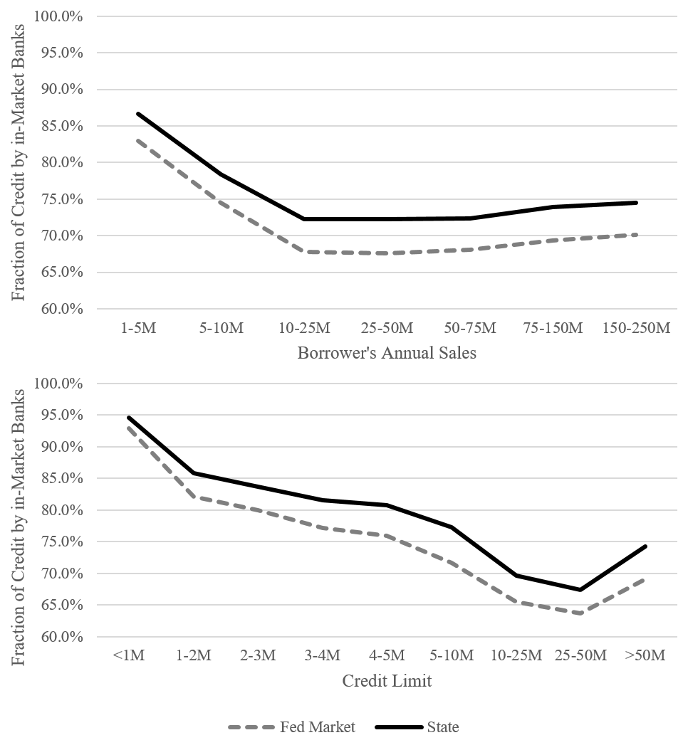
The lower panel of Figure 1 illustrates a strong negative relationship between lender proximity and loan size. The fraction of loans originated by in-market banks decreases sharply as loan size increases until credit lines exceed $50M. This suggests that medium-sized businesses tend to search for lenders more frequently outside their geographic area as loan size increases. This can be rationalized by an external funding premium that is increasing in credit demand, since the opportunity costs of high interest rates or fees increase with the size of the loan. This is also consistent with the view that markets for small business lending are local while the market for large-scale loans is national.
The statistics above show the relationship between firm size and loan size and a middle market borrower's choice of geographically close banks. We naturally expect that firm size is correlated with loan size and, therefore, their raw correlations in the data do not allow us to separately quantify their relationships with lender proximity. To more formally assess borrowers' choice of lenders conditional on other variables, we estimate the following equation using Ordinary Least Squares (OSL). Here, we identify firm size, loan size, expected utilization of the credit line, and market size as the primary determinants of the geographic scope of demand. Formally, we estimate:
$$$$\begin{align} {Local}_{ijt} &= \beta_1 Log({FirmSize})_{it} + \beta_2 Log({TotalCreditLine})_{ijt} + \beta_3 \frac{{UtilizedAmount}_{ijt}}{{TotalCreditLine}_{ijt}} \\\ &+ \beta_4 Log({FedMarketSize})_{ijt} + \beta_5 Log({StateMarketSize})_{ijt} + \varepsilon_{ijt}\end{align}, $$$$
Where $$i$$ is an index for the borrowing firm, $$j$$ is an index for the loan, $${Local}_{ijt}$$ is an indicator variable which equals 1 if the loan is originated by an in-market bank, $$\varepsilon_{ijt}$$ is an error term, and $$\beta$$s are the parameter to be estimated.
Table 4 presents the OLS estimation results, reporting coefficients for firm size, loan size, and credit utilization. The first row measures $${Local}_{ijt}$$ at the Fed market level, and the second row measures $${Local}_{ijt}$$ at the state level. Surprisingly, we find that the results are not sensitive to including controls for market size. The market size variables have positive and statistically significant relationships with lender proximity, as well.
Table 4: Lender Proximity Regression Results
| $${Local}_{ijt}$$ | Log(Firm Size) | Log(Loan Size) | Utilization Fraction |
|---|---|---|---|
| Fed Market Lender | -0.024 | -0.056 | -0.078 |
| (0.002) | (0.001) | (0.003) | |
| State Market Lender | -0.008 | -0.055 | -0.056 |
| (0.002) | (0.001) | (0.003) |
Notes: Both regressions have 77,070 observations (loans) and unreported market size control variables. Standard errors are reported in parentheses; all coefficients are statistically different from 0 at 0.1 % significance level. The adjusted R-squared statistics for in-Fed-market lender and in-State lender models are 0.119 and 0.049, respectively.
The results in Table 4 show, at both the Fed market-level and state-level, that there is negative and statistically significant relationship between choosing an in-market bank and the borrower's scale and loan size. The regression results are consistent with an external funding premium that is increasing in credit demand and increasing in firm scale. The regression results also suggest that the scale relationship is driven by borrower substitution to regional lenders, while most of the loan size relationship is driven by broader regional or national substitution. The latter finding is to be expected, given the lower panel of Figure 1.
Both the firm size and loan size relationships are significant even after controlling for the other variables. However, in terms of magnitude, the results suggest that loan size and expected utilization of the credit line are the primary determinants of the geographic scope of demand. Lender proximity has a negative and statistically significant relationship with the utilized credit fraction, defined as the utilized credit amount divided by the total credit line of the loan. The role of scale in the regression estimates confirms our expectation from the upper panel of Figure 1.
The results presented in Table 4 and Figure 1 are consistent with the hypothesis that firms with larger sales, searching for larger loans, and with higher expected utilization of the loan are more likely to search for lenders in larger geographic scope. This provides heuristic guidance in favor of larger geographic market definitions for loans to medium-sized businesses, especially for borrowers seeking larger loans and expecting more credit utilization. However, most firms still choose an in-market lender. Therefore, the baseline evidence on lender proximity does not endorse broader regional markets over narrow geographic markets, or vice versa, and therefore does not confirm or rule out competitive concerns in middle market lending.
Which Geographic Market Definition?
To formally assess the appropriateness of geographic market definitions for middle market lending, we employ a Hypothetical Monopolist test.4 This test is commonly used by antitrust authorities to establish market definitions for merger proposals. Can a hypothetical monopolist who controls all lenders within the candidate geographic market definition raise an interest rate without losing so many borrowers that such a price increase, a Small but Significant and Nontransitory Increase in Price (SSNIP), would be unprofitable? If the data suggest the SSNIP is unprofitable, then the candidate market is too narrowly defined.
How can the profitability of a SSNIP be measured? The tradeoff between the SSNIP $$x$$ and lost demand $$L$$ depends on the hypothetical monopolist's profit margin $$m=\frac{p-c}{p}$$. In percentage changes, the monopolist breaks even imposing a SSNIP if $$(m+x)(1-L) = m$$. Solving this break even condition provides a formula for “critical loss” $$L=\frac{x}{x+m}$$. If data are available for the “critical loss” version of the hypothetical monopolist test, one compares actual lost demand $$\hat{L}$$ due to the SSNIP with critical loss, and if $$\hat{L} \le L(m,x)$$ then a hypothetical monopolist has incentives to impose the SSNIP and the candidate market definition passes the test. If, instead, one finds that actual loss is greater than critical loss, $$\hat{L} \gt L(m,x)$$, then the candidate geographic market is too narrow. Therefore, three numbers are needed to measure the profitability of the SSNIP: $$(m,x,\hat{L})$$.
Actual lost demand due to the SSNIP is counterfactual. Therefore, the market definition test requires estimating loss $$\hat{L}$$. Because the hypothetical monopolist recaptures medium-sized businesses that switch to alternative lenders inside the market definition, only diversion to lenders outside the candidate market count toward loss. Thus, a close approximation to loss is given by the elasticity of demand $$\epsilon$$ times the percentage change in price $$x$$ times the probability $$D_0$$ that displaced consumers do not switch to some other lender inside the market, formally $$\hat{L} = \epsilon x D_0$$. Because pre-SSNIP must be profit maximizing, the margin and demand elasticity are inversely related, $$m = 1/\epsilon$$, which simplifies the loss formula to $$\hat{L} = x \ D_0/m$$. Comparing estimated loss to critical loss, the hypothetical monopolist test for a candidate geographic market definition is
$$$$ \hat{L} \le L(m,x) \text{ if and only if } D_0 \le \frac{m}{x+m} $$$$
For the diversion ratio to lenders outside the market, $$D_0$$, we use a common estimator that is based on lender choice probabilities, $$\hat{D}_0 = \frac{s_0}{1-s}$$. The aggregate share of out-of-market lenders is $$s_0$$, and the market share of the lender subjected to the SNNIP is $$s$$. Both of these values can be read off the data given a candidate geographic market definition. Diversion is proportional to observed choice probabilities, as we assume, if borrower preferences for one lender over another depend only on ranking those two alternatives relative to each other.5
Lacking data on lender profit margins $$m$$, the last ingredient needed to test the market definition is also counterfactual. To proceed, we compute the smallest margin necessary and sufficient for the candidate geographic market definition to pass the hypothetical monopolist test given values for $$D_0$$ and $$x$$. The margin threshold is an instrument to gauge whether the candidate market is too narrowly defined. A bank's return on assets, though an accounting metric and not a measure of economic profit, is useful to compare to our SSNIP test margins. Banks in the U.S. with more than $15B is assets had an average return on assets of about 1.4 percent (FRED, 2020) over our sample window.
Rearranging the SSNIP test criterion characterizes the general lower bound or threshold margin: $$M \ge x \ D_0/(1-D_0)$$. Plugging in our estimate for $$\hat{D}_0$$, margins must be at least
$$$$ m^{\ast} = x\frac{s_0}{1-s-s_0} $$$$
for all in-market lenders in order for a candidate geographic market definition to pass the hypothetical monopolist test. Since $$m^{\ast}$$ is increasing in the share $$s$$ of the lender affected by the SSNIP, the candidate market definition's minimal passable margin (MPM) is
$$$$ MPM = x \frac{s_0}{1-s_0} $$$$
We conduct the test, estimating MPM and $$m^{\ast}$$, assuming a five percent SSNIP. The MPM is a more lenient criterion, only depends on the out-of-market lender share, and only varies across markets. Since $$m^{\ast}$$ depends on each in-market lender's market share, every market has a distribution of threshold margins. We therefore take the mean of $$m^{\ast}$$ market-by-market and report the between-market variation in SSNIP threshold margins for comparison to the MPM. The results are summarized in Table 5.
Table 5: SSNIP Test Margin Summary Statistics for Fed Markets and States
| Mean | St. Dev. | 10% | 25% | Median | 75% | 90% | |
|---|---|---|---|---|---|---|---|
| Fed market’s MPM | 13.00% | 29.60% | 0.60% | 2.30% | 11.40% | Inf | Inf |
| Fed market’s average m* | 20.80% | 57.70% | 1.80% | 6.00% | Inf | Inf | Inf |
| State’s MPM | 2.90% | 2.50% | 0.80% | 1.40% | 2.00% | 3.90% | 5.60% |
| State’s average m* | 5.00% | 8.80% | 0.90% | 1.60% | 2.30% | 4.40% | 9.60% |
We begin by examining the narrower candidate market definition. The results strongly suggest that Fed markets are too narrow to assess competition in middle market lending. For most Fed banking markets, the threshold margins are too large to be sensible; over half of Fed markets require infinite margins to pass the test. The more lenient MPM measure is kinder to Fed market definitions, but still requires infinite margins from over 25 percent of markets.
Due to these infinite margins, the between-market mean and variance is undefined if geographic markets are Fed markets. Thus in Table 5 we report infinity-censored moments for Fed markets. The censored average margins are 12-13 percent, which we believe is high but still reasonable. These censored averages are driven primarily by MSA Fed markets. Smaller MSA markets have very large test margins, which generates large standard deviations that are approximately twice the scale of the mean. Fed markets defined around large MSAs have sensible results. However, large MSA Fed markets have wider geographic scope than typical Fed markets, and so are closer to a regional market definition and already include more close substitutes than a typical Fed market.
Next we incorporate the next closest substitutes into an expanded candidate market definition, widening the geographic scope of the market to a larger regional area as proxied by states. The state-level results suggests that wider geographic scope is indeed more appropriate for assessing competition in middle market lending. No states have infinite MPM or average threshold margins $$m^{\ast}$$. Therefore, the moments in Table 5 are not censored for state markets. The mean MPM across states is 2.9 percent, and the mean of the stricter SSNIP threshold $$m^{\ast}$$ is 5.5 percent. Nearly all state-based geographic markets have MPMs less than 6 percent. Compared to the Fed market results, between-state variation in SSNIP margins is also closer to the scale of the mean and more symmetrically distributed.
The hypothetical monopolist test results strongly favor larger regional market definitions over Fed banking market definitions for assessing competition in the middle market. However, the results do not necessarily imply that states are themselves the correct market definition. States are only a proxy for regional markets, and there are other possible regional geographic partitions which have not been subjected to the test and compared to our state-level results. However, we believe alternative geographic regions would produce an overall similar distribution of market concentration as the state-based partition. Hence, were we to hone in on a more accurate regional geographic market definition, our conclusion that middle market lending is relatively unconcentrated is unlikely to change.
Borrower Inertia
In the previous sections, we investigate how geographic proximity affects a borrower's lender choice. In this section, we further investigate borrower's choice from the perspective of the frequency of a borrower's lender-switching behavior. Table 6 presents basic statistics on the number of lenders that each borrower has a relationship with. We report the borrower’s total number of lenders, total number of in-state lenders, and the percentage of borrowers who changed lenders between Q4 2017 and Q4 2018.
Table 6: Borrower’s Lender Relationships and Switching Behavior
| Number of Lenders | Number of In-State Lenders | Switched Lenders | |
|---|---|---|---|
| Mean | 1.06 | 0.9 | 4.55% |
| Standard Deviation | 0.37 | 0.44 |
Notes: Calculations based on 49,707 loans observed in both Q4 2017 and Q4 2018.
On average, each borrower only has a credit line from one lender, and most of these lenders are in-state banks. The third column of Table 6 shows that 4.55 percent of middle market firms either switched banks (bank-to-bank substitution), formed a new credit line (outside-to-inside substitution), or destroyed a credit line (inside-to-outside substitution). We observe similar switching rates in prior years. Since the median loan term is seven years for middle market firms, the data imply that middle market firms do in fact search for and switch lenders frequently. About 1/7 = 14 percent of all loans reach maturity each year. A back-of-the-envelope calculation from an overall switching probability of 4.55 percent thus indicates that about 32 percent of borrowers switch lenders at maturity.
This within-borrower analysis suggests that switching costs and other forms of inertia do not encumber middle market firms. In light of the market cross-sectional analysis of competition, farther regional banks are likely close substitutes for geographically near banks for medium-sized businesses who switch lenders. Taken together, this evidence suggests that bank mergers with small effects on regional market structure are unlikely to harm mid-sized firms' access to and costs of capital.
Conclusion
Our findings from the Y14 data suggest that there are unlikely to be competitive concerns in the provision of middle market financial services. Lender choice data support broader geographic market definitions than those suited for analysis of small business credit and consumer deposits. For narrower geographic markets, the profit margins implied by formal hypothetical monopolist tests are implausibly large, a strong indicator such market definitions should be expanded in the case of middle market loans. Broader geographic markets seem to be especially appropriate for larger firms and larger loans, with loan size and expected credit utilization being the key determinants of the geographic scope of lender substitution. Regional market concentration is moderate, at most. Competition appears especially healthy for larger firms and larger loans, who act on their incentives to search more broadly for lenders. Evidence on borrower inertia complements these findings, suggesting that medium-sized businesses' substitution patterns foster rather than impede lender competition.
Our findings support scrutiny of proposed bank mergers that affect concentration at the regional level, since these mergers might impact middle market firms' access to capital markets. Antitrust authorities can likely forgo scrutiny of smaller mergers that only impact market structure locally. Nonetheless, economic policy makers should be mindful of the middle market's regional character, as it could shape a policy's impact on mid-sized firms' access to capital and costs of credit.
Bibliography
Anenberg, Elliot, Andrew C. Chang, Serafin Grundl, Kevin B. Moore, and Richard Windle (2018). "The Branch Puzzle: Why Are there Still Bank Branches?" FEDS Notes. Board of Governors of the Federal Reserve System.
Board of Governors of the Federal Reserve System (2020). "FAQs: How do the Federal Reserve and the U.S. Department of Justice, Antitrust Division, analyze the competitive effects of mergers and acquisitions under the Bank Holding Company Act, the Bank Merger Act and the Home Owners Loan Act?" Retrieved May 2020.
Brevoort, Kenneth P. and Timothy H. Hannan (2006). "Commercial Lending and Distance: Evidence from Community Reinvestment Act Data." Journal of Money, Credit and Banking, 38(8), 1991-2012.
Chernenko, Sergey, Isil Erel, and Robert Prilmeier (2019). "Nonbank Lending." National Bureau of Economic Research, Working Paper #26458.
Elliehausen, G.E. and J.D. Wolken (1990). "Banking Markets and the Use of Financial Services by Small and Medium-Sized Businesses." Federal Reserve Board of Governors Staff Studies, #160.
FDIC (2018). "FDIC Small Business Lending Survey." Federal Deposit Insurance Corporation.
FRED (2020). "Federal Financial Institutions Examination Council (US), Return on Average Assets for U.S. Banks with average assets greater than $15B [USG15ROA]." FRED, Federal Reserve Bank of St. Louis, retrieved April 2020.
Kwast, M., M. Starr-McCluer and J. Wolken (1997). "Market Definition and the Analysis of Antitrust in Banking." The Antitrust Bulletin, 42(4).
Tannenwald, Robert (1994). "The Geographic Boundaries of New England's Middle-Lending Markets." New England Economic Review.
U.S. Department of Justice and Federal Trade Commission (2010). "Horizontal Merger Guidelines."
1. All authors: Federal Reserve Board of Governors, 20th & C St NW, Washington, DC 20551, [email protected], and [email protected]. The analysis and conclusions set forth are those of the authors and do not indicate concurrence by other members of the staff, by the Board of Governors or the Federal Reserve Banks. Return to text
2. These figures, while sizable, establish a lower bound on the economic importance of the middle market, because Y14 reports were only filed by the 30 largest bank holding companies in 2018. Return to text
3. Alternative characterizations of the middle market might focus on loan sizes instead of on firm scale, on assets instead of sales to measure scale, or on a more restricted core range of sales. Instead of adopting such restrictions a priori, we prefer to subsume them and consider narrower notions of the middle market as a robustness exercise. Return to text
4. Antitrust authorities "employ the hypothetical monopolist test to evaluate whether groups of products in candidate markets are sufficiently broad to constitute relevant antitrust markets. … Specifically, the test requires that a hypothetical profit-maximizing firm, not subject to price regulation, that was the only present and future seller of those products ("hypothetical monopolist") likely would impose at least a small but significant and non-transitory increase in price ("SSNIP") on at least one product in the market, including at least one product sold by one of the merging firms. … The hypothetical monopolist test ensures that markets are not defined too narrowly, but it does not lead to a single relevant market. The Agencies may evaluate a merger in any relevant market satisfying the test, guided by the overarching principle that the purpose of defining the market and measuring market shares is to illuminate the evaluation of competitive effects. Because the relative competitive significance of more distant substitutes is apt to be overstated by their share of sales, when the Agencies rely on market shares and concentration, they usually do so in the smallest relevant market satisfying the hypothetical monopolist test. … The hypothetical monopolist's incentive to raise prices depends both on the extent to which customers would likely substitute away from the products in the candidate market in response to such a price increase and on the profit margins earned on those products." (U.S. Department of Justice - Federal Trade Commission Horizontal Merger Guidelines, 2010, Sections 4.1.1 & 4.1.3.) Return to text
5. Formally, we assume that mid-sized firms’ preferences for lenders satisfy the Independence of Irrelevant Alternatives (IIA) property. To illustrate IIA, suppose a borrower prefers lender $$A$$ to lender $$B$$. If the borrower then contemplates a third lender, $$C$$, the IIA property requires that alternative $$B$$ is not chosen. That is, the borrower may or may not prefer $$C$$ to $$A$$, but the ranking of $$A$$ relative to $$B$$ is independent of $$C$$. The SSNIP $$x_i$$ causes some borrowers to switch or divert from lender $$i$$. The IIA assumption implies that diversion $$d_{ik}$$ from lender $$i$$ to lender $$k$$ is equal to the probability that $$k$$ is preferred given that $$i$$ is not chosen, formally expressed $$d_{ik} = s_k / (1-s_i)$$. Total diversion to out-of-market lenders is thus $$D_0 = s_0 / (1-s_i)$$. Return to text
Benson, David, and Ken Onishi (2020). "Are There Competitive Concerns in "Middle Market" Lending?," FEDS Notes. Washington: Board of Governors of the Federal Reserve System, August 10, 2020, https://doi.org/10.17016/2380-7172.2618.
Disclaimer: FEDS Notes are articles in which Board staff offer their own views and present analysis on a range of topics in economics and finance. These articles are shorter and less technically oriented than FEDS Working Papers and IFDP papers.