FEDS Notes
March 05, 2020
Common and idiosyncratic inflation1
Matteo Luciani
One of the major challenges that the Federal Reserve faces in achieving its goal of maintaining price stability is to avoid responding to sector- or industry-specific relative price changes or—even worse—to measurement error. Rather, the Federal Reserve should respond only to macroeconomic shocks, that is, to those shocks that affect all prices and thus change the general price level of goods and services. Thus, determining how much of a current change in prices is driven by macroeconomic factors, as opposed to idiosyncratic developments or measurement error, is a crucial task for the Federal Reserve.
In this note, we disentangle changes in prices due to economy-wide (common) shocks from changes in prices due to idiosyncratic shocks. To do so, we use a new statistical methodology that is entirely data-driven, i.e., it does not make any "structural" economic assumptions or ad hoc judgments about what factors are affecting prices. Indeed, although some idiosyncratic shocks are related to identifiable events (such as changes in Medicare reimbursement rates or one-off changes in the index for wireless telephone services) not all such shocks can be reliably traced to specific developments. Therefore, a statistical model capable of effecting this sort of decomposition is necessary.
The main product of our methodology is a decomposition of the PCE price index excluding food and energy (henceforth "core" PCE). We choose to decompose core PCE prices instead of total PCE prices for a couple reasons. First, although the objective of the Federal Reserve is specified in terms of the inflation rate of the overall PCE price index, food and energy prices can be extremely volatile and therefore "core inflation usually provides a better indicator than total inflation of where total inflation is headed in the medium term" (Yellen, 2015, p. 10). Second, food and energy prices are often driven by idiosyncratic factors that are beyond the influence of monetary policy (Blinder, 1997).
Methodology
Our methodology involves two steps. In the first step, by estimating a dynamic factor model on a dataset of disaggregated PCE prices, we decompose the inflation rate of each item into two components. The first component—the common component—is meant to reflect price changes that are attributable to economy-wide (i.e., common) factors, such as the amount of slack in the economy or movements in the prices of non-labor inputs to production, such as commodity prices, as well as prices of imported goods and services. By contrast, the second component—the idiosyncratic component—is meant to capture relative price movements that reflect sector specific developments, such as the massive decline in prices for wireless telephone services in March 2017, or it can also reflect measurement error, such as sampling error.2
In the second step, after the common components for each individual series have been computed, we aggregate them together to construct the common component of core PCE price inflation by using the series' weights in the overall core PCE price index. This yields an estimate of the portion of core PCE price inflation that can be attributed to common (macroeconomic) factors, which we call "common core inflation."
Empirical analysis
We estimate the dynamic factor model on a dataset of 146 disaggregated monthly PCE prices from January 1995 to June 2019.3 The dataset that we use represents a particular disaggregation of PCE prices in which each disaggregated (or sub) price index is constructed from a distinct data source. Most PCE prices are measured using a corresponding sub-index from the CPI, a few of them are measured using PPIs, and a number of others are imputed. As a result, some disaggregated PCE prices are based on the same CPI (or PPI) series, which means that there are PCE sub-price indexes that are identical (or nearly so).4 To avoid having sub-indexes that are highly correlated by construction, we combine all sub-indexes whose source data is the same.5
We begin by looking at how our model characterizes PCE prices in terms of common and idiosyncratic dynamics. To this end, Table 1 reports the standard deviation of monthly core PCE price inflation (common core inflation) at different frequencies. As we can see, common core inflation accounts for 8.5% of the total variation in core PCE price inflation. However, common core inflation is much less variable at high frequencies, which means that it accounts for more than 18% of the mid- to low-frequency fluctuations (i.e. those with period longer than one year) in core PCE price inflation, and very little of the ultra-high frequency fluctuations with period shorter than six months.
Table 1: Standard deviation of core PCE price inflation and common core inflation
| Overall | $$\tau \ge 60$$ | $$12 \le \tau \lt 60$$ | $$6 \le \tau \lt 12$$ | $$\tau \lt 6$$ | |
|---|---|---|---|---|---|
| $$100 \times \sigma_{\pi^c}^2$$ | 0.612 | 0.055 | 0.090 | 0.094 | 0.391 |
| $$100 \times \sigma_{\chi^c}^2$$ | 0.053 | 0.01 | 0.022 | 0.008 | 0.012 |
| $$ 100 \times \sigma_{\chi^c}^2 / \sigma_{\pi^c}^2 $$ | 8.61 | 18.65 | 24.56 | 8.52 | 3.18 |
This table reports the variance of monthly core PCE price inflation, $$\sigma_{\pi^c}^2$$, and of common core inflation, $$\sigma_{\chi^c}^2$$, at different frequencies. The second column reports the overall variance. The third column reports the variance of fluctuations with period $$\tau$$ longer than 60 months, a.k.a. longer than five years, explained by the common component. The fourth column reports the variance of fluctuations with period between one and five years. The fifth column reports the variance of fluctuations with period between six months and one year. Finally, the sixth column reports the variance of fluctuations with period shorter than six months.
Figure 1 shows the common and idiosyncratic decomposition of monthly core PCE price inflation. In each plot, the red line is common core inflation, that is, the portion of the one-month percent change in the core PCE price index that is attributable to common shocks, while the blue line gives the idiosyncratic component. By construction, these two components sum to overall core PCE inflation, which is shown in the plots as a black line. Finally, the panel on the left covers the period from 2010 to 2019, while the right panel zooms in on the experience of the last two calendar years with 2019 shaded in light blue.
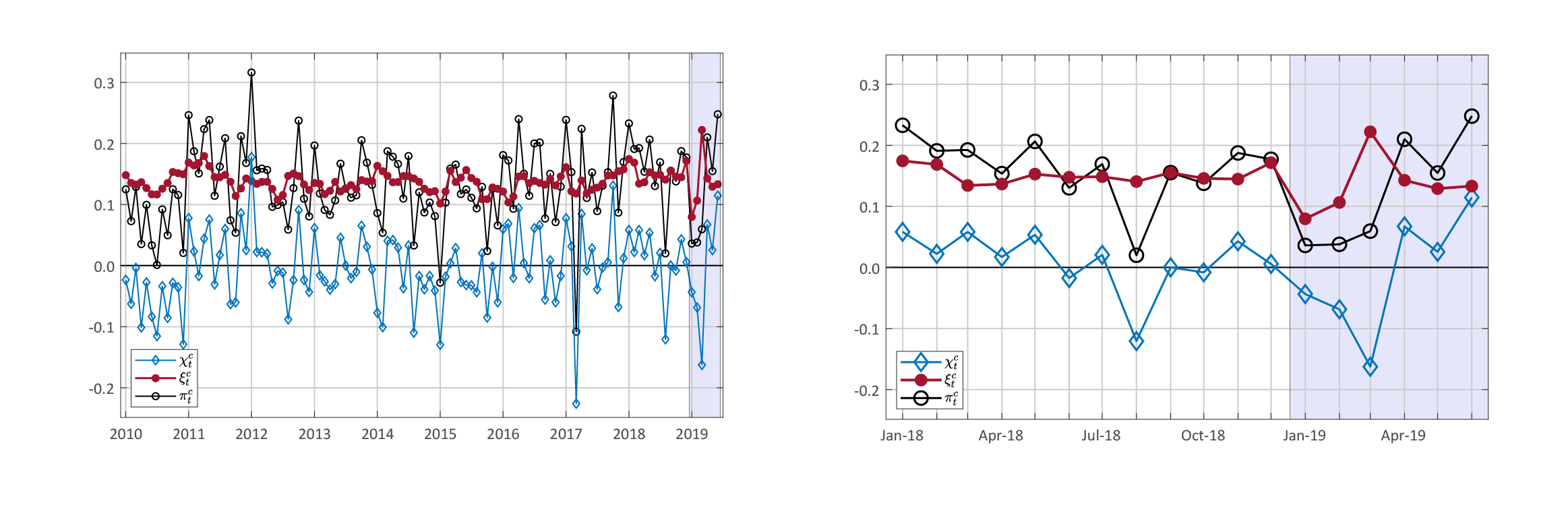
Notes: in each plot, the red line is common core inflation, while the blue line gives the idiosyncratic component. By construction, these two components sum to overall core PCE inflation (the black line). The plot on the left covers the period 2010 to 2019—with 2019 shaded in blue—while the right panel zooms in on the period 2018 to 2019.
By looking at the left plot of Figure 1, we can see that the idiosyncratic component held down core PCE price inflation for most of 2010. Indeed, in 2010 several well-known idiosyncratic negative shocks lowered core inflation, such as the collapse of the index for luggage in January, the very low reading for Medicare hospital services prices in October, and an exceptionally long series of negative readings in the index for apparel. Similarly, idiosyncratic factors held down core inflation in both 2014 and 2015, two years in which medical prices were low in part due to the implementation of the Affordable Care Act. Another episode worth noting is March 2017, when core PCE price inflation was heavily affected by the collapse in the price index for wireless telephone services. Finally, in several years the contribution of the idiosyncratic component is positive at the beginning of the year (in January in particular), while it is negative in the second half of the year, thus showing that the residual seasonality in core PCE prices documented by Peneva (2014) is an idiosyncratic phenomenon.6
Moving to the right panel, we can see that in 2018 idiosyncratic inflation was slightly positive in 9 out of 12 months and strongly negative in August, when prices were held down by, among other factors, the lowest-ever reading for the percent change in the CPI for dental services. As a result, the total contribution of idiosyncratic inflation was nearly zero over 2018 as a whole. Finally, in January, February, and March 2019, idiosyncratic shocks (mainly to non-market-based prices) held down core PCE price inflation by a cumulative 27 basis points, while in April, May and June 2019, they boosted core inflation by a cumulative 20 basis points.
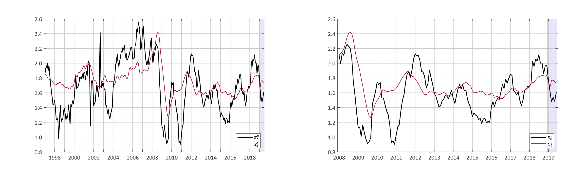
Notes: in each plot, the red line is year-on-year common core inflation, while the black line is year-on-year core PCE price inflation. The plot on the left covers the period 1997 to 2019, while the right panel zooms in on the period 2008 to 2019. The shaded blue area highlights data for 2019.
Figure 2 shows the common and idiosyncratic decomposition of the 12-month percent change in the core PCE price index. Here, the red line denotes year-on-year common core inflation, i.e., the common component's contribution to the overall 12-month percent change of the core PCE price index (which is given by the black line). Put differently, the red line tells us what core inflation would have been had there been no idiosyncratic price shocks over the past 12 months.
As we can see from Figure 2, core PCE price inflation and common core inflation moved largely in sync in 2008 and 2009, when the economy was affected by a large macroeconomic shock, and macroeconomic variation likely dominated idiosyncratic variation in the data. After that, idiosyncratic variation has been more important, and core PCE prices have fluctuated around a fairly stable rate of common core inflation. In particular, our model classifies the 2010 downturn in core PCE price inflation as entirely idiosyncratic, and it also suggests that the 2015 and 2017 downturns in core PCE price inflation were due to idiosyncratic dynamics. As a result, since 2010, while year-on-year core PCE prices inflation fluctuated within a range of 1.2 percentage points, common core inflation fluctuated within a much narrower range of 0.4 percentage point. Hence, these results suggest that most of the swings in core PCE price inflation during the current expansion were mostly idiosyncratic in nature.
Finally, Table 2 shows estimates of a Phillips curve model à la Yellen (2015) from which we can compare the response of core PCE price inflation and common core inflation to changes in economic slack. As we can see, in the shorter term, core common core inflation respond less, but the estimated relationship is strongly statistically significant; in the longer term, however, the response of common core inflation is a bit higher. Moreover, common core inflation responds to economic slack, while the idiosyncratic component does not. That said, even after filtering out idiosyncratic factors, the estimated Phillips curve is extremely flat post-1995.
Table 2. Price inflation Phillips Curve: 1995:Q4—2019:Q2
| Variable | $$\pi_t^c$$ | $$\chi_t^c$$ | $$\xi_t^c$$ |
|---|---|---|---|
| Economic slack: coefficient | -0.051 | -0.031 | -0.009 |
| (-0.03) | (-0.008) | (0.029) | |
| Economic slack: long-run multiplier | -0.067 | -0.075 | -0.01 |
| $$\tau\ ^2$$ | 0.28 | 0.659 | 0.131 |
Notes: The second column reports estimates for core PCE price inflation, $$\pi_t^c$$. The third column reports estimates for common core inflation, $$\chi_t^c$$. The fourth columns reports estimates for the idiosyncratic component of core PCE price inflation, $$\xi_t^c$$. Standard error in parenthesis. For detail on the estimated Phillips curves see the working paper version of this note.
Conclusions
In this note, we disentangle changes in prices due to economy-wide (common) shocks from changes in prices due to idiosyncratic shocks. To do so, we introduce a new statistical model that is entirely data-driven, i.e., it does not make any "structural" economic assumptions or ad hoc judgments about what factors are affecting prices. We estimate the model on a dataset of 146 disaggregated PCE prices from January 1995 to June 2019. Our model classifies as idiosyncratic many well-known episodes, such as the March 2017 collapse in the index of wireless telephone services, and it suggests that most of the fluctuations in core PCE prices since 2010 have been idiosyncratic in nature. Finally, our estimate of the Phillips curve suggest that the flattening of the Phillips curve is not about noise or non-macroeconomic factors.
References
Blinder, A. S. (1997). Measuring short-run inflation for central bankers - commentary. Review, pages 157–160. Federal Reserve Bank of St. Louis.
Peneva, E. (2014). Residual seasonality in core consumer price inflation. FEDS Notes 2014-10-14, Board of Governors of the Federal Reserve System.
Yellen, J. L. (2015). Inflation dynamics and monetary policy. Speech at the Philip Gamble Memorial Lecture, University of Massachusetts, Amherst, Amherst, Massachusetts, September 24, 2015.
1. This note is a shorter and less technical version of Matteo Luciani (2019). “Common and idiosyncratic inflation,” Finance and Economics Discussion Series 2020-024. Washington: Board of Governors of the Federal Reserve System, https://doi.org/10.17016/FEDS.2020.024.Return to text
2. In March 2017 the price index for wireless telephone services plunged 52% (at an annual rate), shaving off about 8 basis points from the monthly percent change in core PCE prices. The plunge was due to both a methodological change to the measurement of wireless services in the CPI and the fact that in late February of 2017 both Verizon and AT&T (which in March 2017 accounted for nearly 70% of wireless subscriptions in the US) brought back unlimited data plans. Return to text
3. The benchmark specification includes one common factor, and each disaggregated price can load the common factor in a time window of three months. Return to text
4. An example is the PCE price index for "New Domestic Autos" (Item: 7), and the PCE price index for "New Foreign Autos" (Item: 8), which are both constructed out of the CPI for "New cars." Return to text
5. For example, we combine the new domestic and new foreign auto sub-indexes into one sub-index on new autos. Return to text
6. A time series suffers from residual seasonality when a predictable pattern occurs over the year, despite the series being previously seasonal adjusted. Return to text
Luciani, Matteo (2020). "Common and idiosyncratic inflation," FEDS Notes. Washington: Board of Governors of the Federal Reserve System, March 5, 2020, https://doi.org/10.17016/2380-7172.2508.
Disclaimer: FEDS Notes are articles in which Board staff offer their own views and present analysis on a range of topics in economics and finance. These articles are shorter and less technically oriented than FEDS Working Papers and IFDP papers.