FEDS Notes
June 07, 2019
Cyclicality and the Severity of the U.S. Supervisory Stress Test: 2014 to 2018
Jose Berrospide, Andrew Cohen, Ronel Elul (Federal Reserve Bank of Philadelphia), David Hou, Aytek Malkhozov, Marc Rodriguez, and Robert Sarama1
In this study, we provide a measure of the severity of the 2014-2018 US supervisory stress tests, and examine how that severity measure has evolved. Since the passage of the Dodd-Frank Act in 2011, large banks (over $50 billion in assets) have been required to undergo supervisory stress tests performed by the Federal Reserve.2 The supervisory stress test provides the public an evaluation of the resilience of the largest banking institutions to prolonged periods of severe stress. It is also used in the Federal Reserve's Comprehensive Capital Analysis and Review (CCAR) to evaluate the ability of firms to make planned capital distributions and remain adequately capitalized during periods of severe stress.3 That is, the amount of capital that banks may distribute to shareholders critically depends on the amount their capital is projected to decline in the supervisory stress test.
A number of factors can affect the size of the projected capital declines in the supervisory stress test. The stress test is a hypothetical exercise that begins from a "jumping off point" characterized by current bank conditions, such as portfolio characteristics, and the broader economic conditions, such as the prevailing unemployment rate and house prices. From that jump-off point, economic conditions are assumed to deteriorate, and models based on historical relationships between elements of the scenario and banking conditions at the jump-off point are used to project the amount each bank's capital would decline. All else equal, a more severe economic scenario will result in larger operating losses and a greater reduction in available capital for the banks, while stronger banking conditions at the jump-off point would have the opposite effect.
Keying the supervisory stress test off of banks' conditions and the broader economic environment at the start of the stress test results in some inherent procyclicality, because, almost by definition, banks will start with stronger portfolios (in terms of recent performance) and revenue profiles during expansions. For instance, financial accelerator dynamics that make borrowers appear to be most creditworthy at the top of the cycle will necessarily result in fewer projected defaults, lower projected losses, and higher projected net income when the starting point for the hypothetical economic stress is closer to the top of the cycle. In order to limit the extent to which the stress tests contribute to this procyclicality, the scenario design framework used by the Federal Reserve contains countercyclical features. Specifically, the macroeconomic stress scenarios are designed to be more severe during expansions and less severe during contractions.
The goal of using countercyclical economic scenarios is to reduce, or ideally remove, the procyclicality of the stress test. Whether the stress tests should be used as an explicitly countercyclical tool, which would involve "overcorrecting" for the inherent procyclicality, is a policy question that is beyond the scope of this note. Instead, our measure of stress test severity, which we can calculate consistently over time, allows us to evaluate how the interaction of procyclical and countercyclical features of the stress test has affected the severity of post-stress outcomes through the current expansion.
Our results may be of particular interest to policymakers looking to integrate the stress tests into other components of the post-crisis regulatory capital regime, such as a stress capital buffer (SCB) and the countercyclical capital buffer (CCyB).4 Because our study evaluates the severity of the supervisory stress test over a period of credit and macroeconomic expansion, it may inform how the two buffers could interact as the business and credit cycles crest. For example, if stress tests conducted in periods where the credit or business cycle is approaching a peak systematically yield more severe results, one might argue that the countercyclical features of the stress test obviate the need for a CCyB. On the other hand, if stress test outcomes are less severe closer to the peak of a cycle, then it could be appropriate to set the CCyB at a higher level than what is suggested by current guidance.5
Broadly speaking, our results indicate that, while it may be possible to use more severe economic scenarios to counteract the procyclical elements of the stress test, it is very difficult to push beyond that in order to engineer countercyclical stress test outcomes. Specifically, while the severely adverse macroeconomic scenario has become more and more unfavorable during the expansion from 2014 to 2018, the "outcomes" of the stress tests have been, if anything, somewhat less constraining to the banks over that same time period. We draw the limited conclusion that using the stress tests as a lever to generate countercyclical capital requirements--if a more countercyclical capital framework were desired by policymakers--is likely not possible without increasing the severity of the stress scenario to levels well beyond those used over the 2014-2018 stress test cycles.
In Section II of this note, we provide a definition of stress test severity that allows us to measure the severity of the test consistently across time-periods. Section III describes the key drivers of stress test severity, and shows how they have changed over time. Section IV shows how our measure of overall stress test severity and its constituent parts have varied over time, and Section V concludes.
II. Measuring stress test severity
There are a variety of ways to measure stress test severity, and no single measure is perfect. In defining a measure, one must decide the relevant "outcome variable" for a stress test, and ways to decompose the factors contributing to that variable.
Media and commentators have traditionally gauged severity by observing how individual firms perform under hypothetical stress scenarios; for instance, the number of firms that fall below minimum regulatory thresholds on a post-stress basis.6 Other studies have focused on the severity of the economic scenarios (Liang 2018, Durdu, Edge, and Schwindt 2017, and Glasserman and Tangirala 2015). More recently, studies focus on the decline in capital ratios during the projection horizon (Cortés, Demyanyk, Li, Loutskina and Strahan 2018, Berrospide and Bassett 2018, Covas 2018). This latter measure has the benefit of including all potential drivers of changes in severity of the stress test. For example, it incorporates the effects of changes in models and changes in scenarios. However, the measure also includes changes in planned capital distributions from year to year.
Another simple way to measure the severity of the stress tests, emphasized here, is to calculate the total decline in common capital ratios from the beginning to the end of the projection horizon, after netting out planned capital distributions. We focus on this metric for two reasons. First, ending capital ratios facilitate comparability across time. Regulatory capital minimums can occur in different projection quarters depending on a variety of factors including firms' business models, the amount and timing of planned capital distributions, and the phase-in of U.S. regulatory capital rules. Standardizing the analysis to the full nine-quarter projection horizon ameliorates these year-over-year differences.7 Second, the stress tests serve to limit the amount of capital a firm can distribute by requiring firms to meet post-stress minimum capital requirements. Thus, we think it most appropriate to focus on the portion of the decline in capital that represents a possible constraint on a firm's capital distributions. To put it another way, we think that two stress test exercises where there is a $100 decline in Common Equity Tier 1--one in which firms made no capital distributions and one in which the entire $100 decline was due to planned capital distributions--are not equally "severe."
III. Factors that can change stress test severity
Before presenting our results on overall stress test severity, we describe how the severely adverse stress scenario as well as bank portfolio conditions and profitability have changed over time. Although other factors have influenced stress test severity over time, those have been less impactful and are not explicitly tied to either the business or credit cycle.8
Changes in the macroeconomic scenario
The scenario design process for the Federal Reserve's supervisory severely adverse scenario has a number of countercyclical features. Most importantly, the unemployment rate is constrained to reach a level of at least 10 percent in the severely adverse scenario, regardless of the current rate of unemployment. Because remaining scenario variables are chosen in a manner such that they are consistent with a well-specified model of the macroeconomy, the larger changes in the unemployment rate required when the starting rate for unemployment is low will generally result in more significant changes to the other scenario variables, and hence more countercyclical scenarios. For example, a more significant decrease in GDP would be expected in a stress test where unemployment increased by 6 percentage points to 10 percent as opposed to a test in which unemployment increased by 4 percentage points to 10 percent.
As shown by table 1, the severity of the scenarios measured as the changes in key variables from start to trough has been increasing between 2014 and 2018. For example, the BBB-bond rate spread widened just 3 percentage points in 2014 compared to a 4.25 percentage point widening in 2018.
Table 1: Certain Scenario Variables, Supervisory Severely Adverse Scenario, CCAR 2014 to CCAR 2018
| 2014 Severely Adverse | 2015 Severely Adverse | 2016 Severely Adverse | 2017 Severely Adverse | 2018 Severely Adverse | |
|---|---|---|---|---|---|
| Unemployment rate | ↑4 p.p.to 11-1/4% | ↑4 p.p.to 10% | ↑5 p.p.to 10% | ↑5-1/4 p.p.to 10% | ↑5-3/4 p.p.to 10% |
| House prices | ↓25% | ↓25% | ↓25% | ↓25% | ↓30% |
| CRE prices | ↓35% | ↓35% | ↓30% | ↓35% | ↓40% |
| BBB-bond rate spread | ↑3 p.p.to 5 p.p. | ↑3-1/2 p.p.to 5 p.p. | ↑3-1/2 p.p.to 5-3/4 p.p. | ↑3-1/2 p.p.to 5-1/2 p.p. | ↑4-1/4 p.p.to 5-3/4 p.p. |
| Equity prices | ↓50% | ↓60% | ↓50% | ↓50% | ↓65% |
Source: Board of Governors of the Federal Reserve System, “Supervisory Scenarios for Annual Stress Tests Required under the Dodd-Frank Act Stress Testing Rules and the Capital Plan Rule” (Washington, DC: Board of Governors) for the years 2014 through 2018, available at https://www.federalreserve.gov/supervisionreg/ccar.htm.
Figure 1 shows the paths of two important variables--the unemployment rate and house prices--in the macroeconomic scenario over the past several years. Consistent with the Federal Reserve's publicly available scenario design framework, the unemployment rate in the severely adverse scenario rises to at least 10 percent.9 As seen in the left panel of figure 1, over the past four exercises the peak of the unemployment rate in the severely adverse scenario occurs at 10 percent.
Similarly, as shown in the right panel of figure 1, in the past few cycles house prices have fallen to a similar trough in the Federal Reserve's severely adverse scenario even though starting house prices (black line) have risen at a steady clip during that time period.10
The interest rate component of the scenarios is also a key driver of changes in projections from year to year, as it affects projections of revenues and the values of assets that are measured at fair value. In recent years the interest rate variables have been specified to capture salient risks, such as negative short term rates in 2016 or a global aversion to long-term, fixed-income assets in 2018.
Figure 1: Paths of Unemployment Rate and House Prices, Actual and Supervisory Severely Adverse Scenario, CCAR 2014 to CCAR 2018
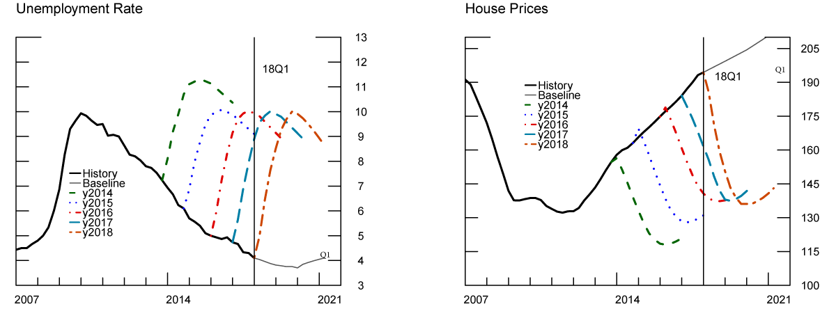
Source: Board of Governors of the Federal Reserve System, “Supervisory Scenarios for Annual Stress Tests Required under the Dodd-Frank Act Stress Testing Rules and the Capital Plan Rule” (Washington, DC: Board of Governors) for the years 2014 through 2018, available at https://www.federalreserve.gov/supervisionreg/ccar.htm. Historical paths are based on the latest data release. The differences between past scenario jump-off points and historical values reflect data revisions released after the publication of the respective scenario.
Changes in portfolio conditions and profitability
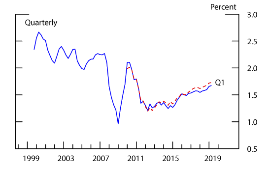
Portfolio conditions have generally improved due to a combination of a healthier economy and improved underwriting standards earlier this decade, and that is evident even in simple measures of risk, such as the share of delinquent loans. In figure 2, we show the delinquency rate on loans at the balanced panel of banks that have participated in CCAR continuously since 2014. The hangover of delinquent loans from the financial crisis was still evident in loan portfolios in 2014 but has since subsided. The reduction in delinquency rates is due in large part to improved economic conditions such as rising real estate prices, narrowing corporate debt funding spreads, and lower unemployment rates.
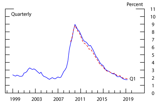
Profitability at banks is also procyclical, and all else equal more-profitable banks have smaller post-stress declines than less-profitable banks. Pre-provision net revenue (PPNR) is a measure of profitability that removes the effect of loan loss provisions. It is equal to net interest income plus noninterest income minus noninterest expense, which is the primary source of net income, and therefore a key component in banks' post-stress capital ratios. In figure 3, we show trailing four-quarter PPNR (normalized by average assets) at the balanced panel of banks that have participated in CCAR continuously since 2014. That measure of bank profitability has risen at a fairly steady pace over the past five years.
Source: FR Y-9C. The red dashed line includes the full set of banks continuously subject to the supervisory stress test since 2014. The blue line includes the subset of those banks for which FR Y-9C data are available from 1998q4 to present. Delinquency rate is defined as balance of loans 30 days past due or in nonaccrual divided by total loan balances.
Source: FR Y-9C. The red dashed line includes the full set of banks continuously subject to the supervisory stress test since 2014. The blue line includes the subset of those banks for which FR Y-9C data are available from 1998q4 to present. PPNR is defined as net interest income plus noninterest income minus noninterest expense.
IV. Severity of the stress test over time
The supervisory stress tests measure firms' capital resiliency using six different capital ratios at various points in time.11 We focus on the decline in the common equity ratio, which is generally considered the most loss-absorbing measure of capital.12 Common equity is best measured using the tier 1 common ratio in the 2014 and 2015 stress test exercises when Basel I was in effect. The Basel III common equity tier 1 ratio is the best measure afterwards.13
The total decline in the common equity ratio from the beginning to the end of the projection horizon in the five most recent stress test exercises is shown in figure 4 as the combined height of the dark and light blue bars. By this metric, the decline in the common equity ratio in the 2018 exercise was the largest to date. However, a large proportion of this decline is due to planned capital distributions, shown in light blue. Overall stress test severity in 2018, measured as the decline in capital once distributions are netted out, was in line with previous years. The decline in capital excluding distributions, shown in dark blue, equaled 2.7 percent in 2018. This decline exceeds the 2017 value, but is below the overall average of 3 percent, shown by the dashed line. Therefore, by this measure, there is no discernable upward trend in overall stress test severity.
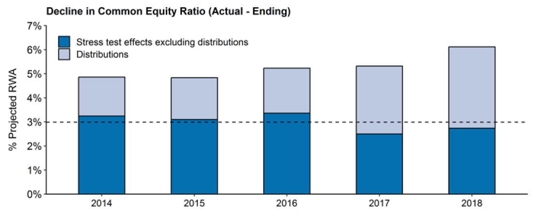
Note: Sample includes a balanced panel of the 28 firms that have participated in the stress tests since 2014. Values are taken under the Supervisory Severely Adverse scenario. The dashed line represents the average non-distribution stress test effect observed in CCAR 2014 through 2018. Capital is measured using tier 1 common in 2014 and 2015, and CET1 thereafter. RWA is measured using the generalized approach for 2015 and 2015, and the standardized approach thereafter. Key identifies bar segments in order from bottom to top.
Source: Staff estimates derived from CCAR results.
Decomposition of overall stress test severity
Figure 5 decomposes the dark blue portion of the bars in figure 4 into separate contributions from balance sheet growth assumptions, regulatory capital deductions and taxes, unrealized losses on securities, and pre-tax net income.
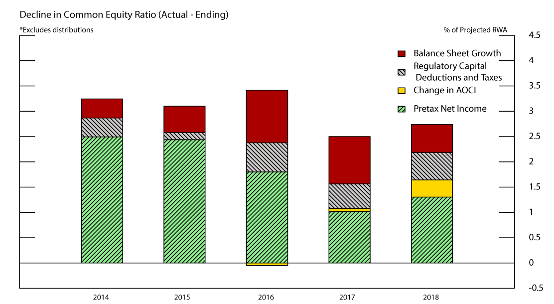
Note: Sample includes a balanced panel of the 28 firms that have participated in the stress tests since 2014. Values are taken under the Supervisory Severely Adverse scenario. The dashed line represents the average non-distribution stress test effect observed in CCAR 2014 through 2018. Capital is measured using tier 1 common in 2014 and 2015, and CET1 thereafter. RWA is measured using the generalized approach for 2014 and 2015, and the standardized approach thereafter. AOCI does not flow through tier 1 common.
Source: Staff estimates derived from CCAR results.
Variation in pre-tax net income (green section of the bars) from year to year is a key driver of variation in stress test severity over time. The pre-tax net income effect is larger in 2018 than in 2017, in part reflecting the effect of a more severe scenario in 2018. However, the pre-tax net income effect is significantly smaller than it was in the supervisory stress tests conducted in 2014, 2015, and 2016. Variation in projected pre-tax net income from year to year reflects differences in portfolio conditions and the effect of macroeconomic and financial conditions in the severely adverse scenario such as falling asset prices, rising equity market volatility, and sharply contracting economic activity. The largest drivers of changes in pre-tax net income are changes in loan losses and PPNR.14 Figures 6a and 6b plot those components over the past several stress test cycles.
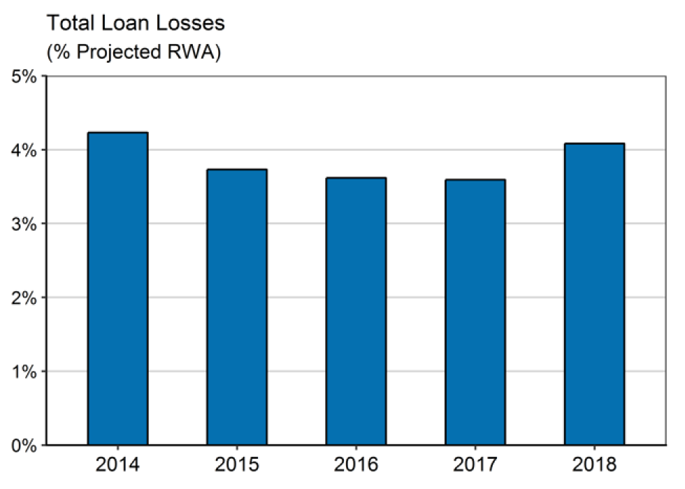
Note: Sample includes the 28 banks that have participated in all CCAR exercises since 2014. The values are taken under the Supervisory Severely Adverse scenario.
Source: Publicly disclosed DFAST results.
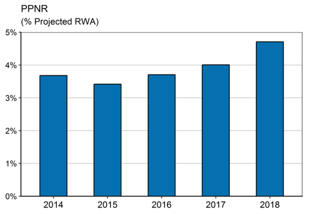
Note: Sample includes the 28 banks that have participated in all CCAR exercises since 2014. The values are taken under the Supervisory Severely Adverse scenario.
Source: Publicly disclosed DFAST results.
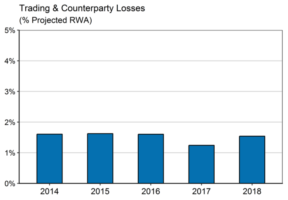
Note: Sample includes the 8 domestic LISCC firms. The values are taken under the Supervisory Severely Adverse scenario.
Source: Publicly disclosed DFAST results.
Notes: Sample includes the 28 banks that have participated in all CCAR exercises since 2014. The values are taken under the Supervisory Severely Adverse scenario.
Source: Publicly disclosed DFAST results.
Total loan losses as a percent of risk-weighted assets (RWAs) fell from the 2014 to the 2015 exercises, in part driven by improvement in balance sheets resulting from banks charging off delinquent, crisis-era loans (see figure 2). Since then, the countercyclical elements of the scenario (see figure 1), along with a shift in lending by these banks to riskier segments (such as credit cards, corporate loans and commercial real estate) have kept it from falling further. The larger increase in 2018 can be generally attributed to the more severe scenario in that year. PPNR relative to RWAs has risen steadily since 2015, reaching its highest level in CCAR 2018. That rise in PPNR in part reflects improvements in bank profitability in recent years (see figure 3), but changes in the interest rate component of the scenarios are also a key driver of changes in PPNR projections in recent years. The 2016 severely adverse scenario featured negative rates on short-term Treasuries, which put downward pressure on net interest income. In contrast, the 2018 severely adverse scenario featured a global aversion to long-term fixed-income assets. That feature translated to a steeper yield curve, which generally bolsters net interest income.
Projected unrealized gains and losses on securities are recognized in the accumulated other comprehensive income (AOCI) component of regulatory capital for the largest firms. The effect of projected unrealized gains and losses on securities on stress test severity is shown in yellow in figure 5, and that effect increased meaningfully in 2018 owing in part to wider corporate bond spreads and no decline in long-term treasury rates. The 2014 and 2015 results show no impact of unrealized losses, as the tier 1 common ratio under the Basel I regime did not recognize unrealized securities gains and losses in regulatory capital.
The effect of balance sheet growth, shown in red in figure 5, also varies from year to year. Supervisory projections of balance sheet growth are primarily driven by historical data on balance sheet growth and changes in supervisory scenarios. These effects vary significantly over time and they helped moderate the capital ratio decline in 2018 relative to the 2017 exercise. Absent the smaller effect of balance sheet growth, the pre-distribution capital ratio decline in 2018 would have exceeded that in the 2017 exercise.15
Finally, regulatory capital deductions and taxes, shown in the grey bars, capture several subcomponents and have remained broadly stable over time. The larger effect in CCAR 2018 in part reflects the effect of changes in the tax code. While the Tax Cuts and Jobs Act reduced the corporate tax rate, it also eliminated the extent to which losses can be used to offset past and future taxes. As a result of that change under the new law, banks that are projected to have losses in the stress test no longer receive as large a tax benefit in the severely adverse scenario as previously.
Concluding remarks
Bank conditions naturally improve during economic expansions because income and growth opportunities increase, the stock of bad loans left over from the previous recession decreases, and borrowers’ economic conditions are generally strong. The stress test scenarios are designed, in part, to offset some of this improvement. However, our measure of stress test severity suggests that the progressively more stringent scenarios during the recent economic expansion have only partially leaned against the procyclicality that has arisen from the recent improvements in bank conditions.
References
Basset, William and Jose Berrospide (2018). "The Impact of Post Stress Test Capital on Bank lending," FEDs WP-087. Washington: Board of Governors of the Federal Reserve System, May 5, 2017, https://doi.org/10.17016/FEDS.2018.087
Covas, Francisco (2018). "A proposal to improve the transparency of stress scenarios" Bank Policy Institute, Research Note, November 13, 2018
Durdu, Bora, Rochelle Edge, and Daniel Schwindt (2017). "Measuring the Severity of Stress-Test Scenarios," FEDS Notes. Washington: Board of Governors of the Federal Reserve System, May 5, 2017, https://doi.org/10.17016/2380-7172.1970.
Glasserman, Paul and Gowtham Tangirala (2015). "Are the Fed's Stress Test Results Predictable?"
The Journal of Alternative Investments Spring 2016, 18 (4) 82-97; https://doi.org/10.3905/jai.2016.18.4.082
Kristle Cortés, Yuliya Demyanyk, Lei Li, Elena Loutskina, and Philip E. Strahan (2018) "Stress Tests and Small Business Lending," NBER Working Paper No. 24365. https://www.nber.org/papers/w24365
Liang, Nellie (2018). "Well-designed stress test scenarios are important for financial stability," The Brookings Institution. https://www.brookings.edu/research/well-designed-stress-test-scenarios-are-important-for-financial-stability/
1. The analysis and conclusions set forth are those of the authors and do not represent the views of the Board of Governors of the Federal Reserve System or others within the Federal Reserve System. The authors are grateful for the helpful comments from Bill Bassett, Bora Durdu, Luca Guerrieri, Kathleen Johnson, Kevin Kiernan, Michael Kiley, Andreas Lehnert, Candy Martinez, Palmer Osteen, Lisa Ryu, and Ahmad Yusuf. Return to text
2. For more information on the Dodd-Frank Act supervisory stress testing requirements, see 12 USC 5365(i)(1). The Federal Reserve Board recently proposed to revise its stress testing rules to account for the higher asset thresholds for the application of the supervisory stress test that were prescribed in the Economic Growth, Regulatory Relief, and Consumer Protection Act (EGRRCPA). Under that legislation, only firms with more than $100 billion in assets will be subject to supervisory stress testing requirements. Return to text
3. For more information on the capital plan rule, see 12 CFR 225.8. Return to text
4. The "stress capital buffer," or SCB, calibrates the current capital conservation buffer to be the minimum of 2.5 percentage points or the stress-test capital buffer, measured in a way similar to the one we consider in this note. For details, see press note released for public comment in April 2018, which can be found at https://www.federalreserve.gov/newsevents/pressreleases/bcreg20180410a.htm. The CCyB is discussed in detail in the Federal Reserve's policy statement, which can be found at https://www.federalreserve.gov/newsevents/pressreleases/bcreg20160908b.htm. Return to text
5. The Federal Reserve's policy statement indicates that it would envision activating to the CCyB to a positive level when financial system vulnerabilities are "meaningfully above normal." Return to text
6. See for example: "Fed toughens stress tests scenarios for 2018" by the American Banker, February 1, 2018, which can be found athttps://www.americanbanker.com/news/fed-toughens-stress-test-scenarios-for-2018, and "Ensuring stress tests remain effective," Money and Banking, January 22, 2018, which can be found athttps://www.moneyandbanking.com/commentary/2018/1/21/ensuring-stress-tests-remain-effective Return to text
7. An alternative approach would be to use the start-to-minimum decline. Such an approach may better characterize the overall severity of the stress test. However, it complicates the decomposition of the drivers from year to year. For the U.S. supervisory stress tests between 2014 and 2018, the start-to-minimum metric for the aggregate set of firms does not result in a materially different contour or level of stress test severity relative to start-to-ending. Return to text
8. For example, enhancements to the supervisory modeling framework have generally been modest, while Basel III phase-ins resulted in somewhat larger capital declines. The Tax Cuts and Jobs Act (TCJA) also led to larger declines in the 2018 exercise, as discussed in the DFAST 2018 disclosure paper. The higher losses in 2018 were attributable to the elimination of carrybacks for net operating losses, which had had a countercyclical effect on capital in stress tests. For more information, see https://www.federalreserve.gov/publications/files/2018-dfast-methodology-results-20180621.pdf Return to text
9. For the policy statement on the scenario design framework for stress testing, see Federal Register document at https://www.federalregister.gov/documents/2017/12/15/2017-26858/policy-statement-on-the-scenario-design-framework-for-stress-testing Return to text
10. In February 2019, the Federal Reserve amended its scenario design policy to introduce a quantitative guide for the house price path in the stress test scenarios. The guide is informed by the ratio of nominal house prices to nominal per capita disposable income. For more information, see https://www.federalregister.gov/documents/2019/02/28/2019-03504/amendments-to-policy-statement-on-the-scenario-design-framework-for-stress-testing Return to text
11. Tier 1 common ratio, common equity tier 1 ratio, tier 1 capital ratio, total risk-based capital ratio, tier 1 leverage ratio, and supplementary leverage ratio. The tier 1 common ratio operated exclusively under the Basel I regime, while the common equity tier 1 ratio and supplementary leverage ratio operated exclusively under the Basel III regime. All other ratios have parallels under both Basel I and Basel III. Return to text
12. As described in "The Supervisory Capital Assessment Program: Overview of Results" (May 7, 2009), because common equity is the first element of the capital structure to absorb losses, it offers protection to more senior parts of the capital structure and lowers the risk of insolvency. Return to text
13. Even though certain firms were subject to Basel III in the 2014 and 2015 exercises, the tier 1 common ratio remained binding for most firms in those two years because valuation allowances on deferred tax assets had not yet been fully introduced into the regulatory capital calculation, and Basel III regulatory capital deductions were gradually phased in over time. Return to text
14. Other drivers of changes in pre-tax net income include trading and counterparty losses and losses from securities portfolios. Return to text
15. The Federal Reserve's stress capital buffer (SCB) proposal assumes that firms' balance sheets remain constant under stress. All else equal, overall stress test severity as measured by the decline in the common equity ratio from the beginning to the end of the stress test exercise would be smaller had the SCB been in effect. See https://www.federalreserve.gov/newsevents/pressreleases/bcreg20180410a.htm. Return to text
Berrospide, Jose, Andrew Cohen, Ronel Elul, David Hou, Aytek Malkhozov, Marc Rodriguez, and Robert Sarama (2019). "Cyclicality and the Severity of the U.S. Supervisory Stress Test: 2014 to 2018," FEDS Notes. Washington: Board of Governors of the Federal Reserve System, June 7, 2019, https://doi.org/10.17016/2380-7172.2393.
Disclaimer: FEDS Notes are articles in which Board staff offer their own views and present analysis on a range of topics in economics and finance. These articles are shorter and less technically oriented than FEDS Working Papers and IFDP papers.