FEDS Notes
September 19, 2025
Evaluating Empirical Regularities in Variable Comovement in Stress Test Scenarios
Elena Afanasyeva, William Bassett, Bora Durdu, Sam Jerow, and Fiona Waterman1
Introduction
Each year, the Federal Reserve Board conducts a stress test of large banks to assess their ability to withstand economic downturns while continuing to lend and meet their obligations. These stress tests include severely adverse scenarios which feature 13-quarter paths of key macroeconomic and financial variables that factor into the calculation of projected capital losses of the stress-tested institutions.2 These variables cover broad categories describing economic and financial developments within the United States: real activity, asset prices or financial conditions, and interest rates.3 This note examines the empirical regularities in the comovement patterns among key domestic variables in the Board's macroeconomic scenario design framework, with the aim of assessing the plausibility of stress test scenarios.
We focus on a subset of domestic variables that are chosen to represent the broader categories covering economic and financial conditions: the unemployment rate, BBB spreads (BBB corporate bond yield less the 10-year Treasury yield), the VIX, commercial real estate (CRE) prices, and equity prices.4 These variables were selected due to their significance in representing different aspects of economic and financial stress. The results obtained for these variables highlight more generally how a number of variables from these broader categories comove in the historical data, and whether the comovement featured in the stress test scenarios is generally comparable to that observed historically.
First, we compare a typical (average) scenario path of the key domestic variables against their corresponding paths observed during the 2007-2009 financial crisis. Second, we use a vector autoregression (VAR) exercise to study how the variables of interest respond to a financial shock and validate our findings with several robustness exercises.
Typical Comovement of Variables in the Past Stress Tests and during the 2007-2009 Financial Crisis
The Board employs a recession approach to specify the paths of variables in the stress test scenarios.5 This approach ensures that stress test scenarios include conditions that typically occur in recessions—such as increasing unemployment, declining asset prices, and contracting loan demand—and can put significant stress on firms' balance sheets.6 To examine the empirical plausibility of such comovement, or how the variables of interest move in relation to each other, we first compare variable trajectories in a stress test scenario to their behavior during a severe recession, e.g., the 2007-2009 financial crisis. The goal of this comparison is to study whether the variables of interest in the stress test scenarios comove similarly to their counterpart in the data, both qualitatively (directionally) as well as quantitatively (by similar magnitudes as implemented in the past stress test scenarios).
A typical trajectory in the stress test scenarios is computed as the average across the published severely adverse scenarios in 2014-2025.7 This approach of using an average scenario is sensible as it provides a representative view of the stress scenarios over time, smoothing out any year-specific scenario choices. In doing so, it allows for a more robust comparison with historical data by capturing the overall severity and pattern of stress envisioned in stress test scenarios across multiple years. For the empirical counterpart to the scenario trajectory, we use the 13 quarters of historical data (to match the length of the scenario) during the 2007-2009 financial crisis, with the jump-off value in 2008Q2 — the quarter preceding the Lehman bankruptcy. The Lehman Brothers bankruptcy on September 15, 2008 is often considered to be the most significant of the events that roiled financial markets during the 2007-2009 financial crisis and is therefore a natural timing cut-off point signifying the triggering event in this crisis.8
The results of this comparison are plotted in Figure 1. Panel (a) shows the comparison for the unemployment rate. The average scenario trajectory is quantitatively very close to its historical benchmark in many respects: its smooth hump-like shape, both the magnitude and the timing of the peak, and the gradual decline after the peak. The recovery phase in the data appears to be somewhat slower with the end value being slightly higher than in the typical scenario.
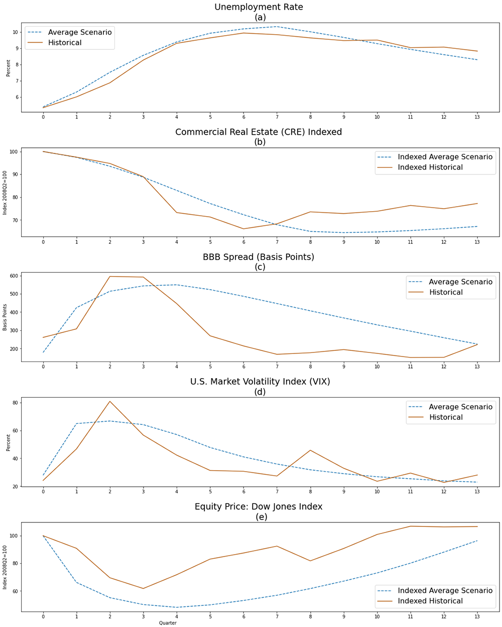
Notes: Historical data starts in 2008 Q2. Scenario averages are computed for scenario paths in 2014-2025.
Sources: U.S. unemployment rate: Quarterly average of seasonally adjusted monthly unemployment rates for the civilian, non-institutional population aged 16 years and older, Bureau of Labor Statistics (series LNS14000000); U.S. Commercial Real Estate Price Index: Commercial Real Estate Price Index, Z.1 Release (Financial Accounts of the United States), Federal Reserve Board (series FL075035503.Q divided by 1000); U.S. BBB corporate yield: Quarterly average of daily ICE BofAML U.S. Corporate 7-10 Year Yield-to-Maturity Index, ICE Data Indices, LLC, used with permission (C4A4 series); U.S. 10-year Treasury yield: Quarterly average of the daily yield on 10-year U.S. Treasury notes, constructed by Federal Reserve staff based on the Svensson smoothed term structure model (see Lars E. O. Svensson, 1995, “Estimating Forward Interest Rates with the Extended Nelson–Siegel Method,” Quarterly Review, no. 3, Sveriges Riksbank, pp. 13–26); U.S. Market Volatility Index (VIX): VIX converted to quarterly frequency using the maximum close-of-day value in any quarter, Chicago Board Options Exchange via Bloomberg Finance L.P; U.S. Dow Jones Total Stock Market (Float Cap) Index: End-of-quarter value via Bloomberg Finance L.P.
Panel (b) of Figure 1 shows the comparison for the CRE prices. Many similarities between the data and the typical scenario trajectory are evident. The magnitude of the decline at the trough as well as a rather sluggish pattern of recovery stand out in both the data and the scenario path. The timing of the trough is slightly earlier in the data than in a typical scenario, and the end value in the data is somewhat higher. The faster recovery in the historical data could be due to the implementation and spillovers of various government programs that were enacted in response to the crisis. Specifically, the Department of the Treasury in conjunction with the Federal Reserve Board launched the Term Asset-Backed Securities Loan Facility (TALF) to help small business credit needs by supporting issuance of asset backed securities (ABS) and commercial mortgage-backed securities (CMBS).9 However, stress test scenarios are constructed to assess the effects of stress on the banks in absence of such government support.10
The typical scenario trajectory of the BBB spread shares several common features with the data as well (panel (c) of Figure 1). The magnitude of the peak in the historical time series (about 600 basis points) is quite similar to the typical peak magnitude in the scenarios (about 550 basis points). For a typical stress test scenario, reaching such a peak would require about 400 basis points increase in the spread from the jump-off point. Both the data and the scenario trajectory display a frontloaded pattern of spread increase to the peak, with the largest share of the increase occurring early on. The end values happen to align very closely between the data and the typical scenario, although the post-peak trajectory to the end values is smoother in the scenario compared with the data. Again, an important difference between the scenario design and the historical experience is in the presence of government support programs in the latter.
Panel (d) of Figure 1 displays the results for the VIX. The frontloaded increase to the peak is similar between the data and the typical scenario trajectory, as is the timing of the peak – in the second quarter. The magnitude of the peak in the 2007-2009 financial crisis is somewhat higher than the one of the average scenario (about 80 percent and 67 percent, respectively), albeit quantitatively not too far apart. While the end values of the trajectories are broadly similar, the post-peak path to them is somewhat less smooth in the data, displaying a zig-zag rather than a steady gradual decline pattern. Furthermore, the recovery starts faster in the data, likely reflecting (among other things) the government support programs announced and implemented at the time – features that are by construction absent in a scenario.
The comparison for equity prices (based on the Dow Jones price index series) is displayed in panel (e) of Figure 1. Both the historical data and the scenario share a frontloaded pattern of the decline to the trough, with the trough in the data sitting somewhat higher in the case of the data (about 40 percent below the jump-off point) compared to the typical scenario (about 50 percent from the jump-off point). The timing of the trough in the scenarios is delayed by one quarter relative to the data. Perhaps for similar reasons of ongoing government support, the recovery of equity prices is somewhat less sluggish in the data, with the end point sitting somewhat higher as well, compared to a typical stress test scenario.
Overall, this simple comparison provides initial evidence in support of the comovement of the variables in the stress test scenarios, both qualitative (directional) and quantitative. In particular, the peak and trough values achieved during the crisis illustrate by how much the variables of interest can change in a well-known historical stress episode. Admittedly, this comparison focuses on just one, albeit prominent episode of financial stress. And, as pointed out above, in contrast with the stress test scenario environment, the presence of government support in response to the crisis can be a likely contaminant of the variable trajectories in the data, especially in recovery phases of the trajectories. Therefore, the next section focuses on a different quantitative exercise, that does not solely rely on the 2007-2009 financial stress experience and that examines the conditional behavior of variables, i.e., their behavior in response to a financial shock – a trigger of financial stress.
Illustrative Exercise with a Vector Autoregression (VAR)
We use a VAR to understand the comovement of variables in the data, as it estimates a system of all variables jointly and can therefore account for variable interactions contemporaneously as well as over time. This approach allows us to capture complex interactions and feedback effects between variables, providing a more comprehensive view of how they move together in response to shocks. Consistent with the earlier exercise, the baseline VAR includes the same key domestic variables: the unemployment rate, commercial real estate (CRE) prices, the corporate BBB bond spread, VIX, and equity prices (S&P 500 Composite Index).11 Before estimation, both CRE and equity prices are transformed by using the log level of the series; no transformations are applied to the other three variables in the system. This treatment of the variables is standard in the Bayesian VAR literature; see Giannone et al. (2015), for example.
This exercise uses the largest available common sample for estimation to include as many observations as possible and increase the precision of the resulting estimates. This estimation sample ranges from 1971Q3 to 2019Q4. To extend the sample size, we use the imputed measure of equity market volatility (rather than VIX) and an alternative measure of the BBB spread.12 As shown in the Appendix (Figures A and B), when plotted over the common sample, both the imputed measure of equity market volatility and the alternative measure of the BBB spread display a high correlation with their respective counterparts. Notably, the VIX measure is somewhat more volatile than the imputed measure. The standard deviation of the VIX is about 1.5 times higher than the standard deviation of the imputed measure, when compared over the common sample of 1990Q1 to 2019Q4.
We estimate the VAR with Bayesian methods, using the prior and the prior hyperparameter selection procedure of Giannone et al. (2015) and imposing a lag order of five quarters – a common choice in the literature for data of quarterly frequency.13 VARs are densely parameterized systems, whereas samples of macroeconomic data are often (also in our case) constrained by data availability and data frequency. Each additional variable (and its lags) included in the VAR system dramatically increases the number of parameters to be estimated and reduces the reliability of the estimates. The prior selection procedure of Giannone et al. (2015) is known to reduce estimation uncertainty and make inference more stable for sample sizes used in macroeconomic applications. This feature is particularly relevant in our case, as we apply the methodology of Giannone et al. (2015) in the threshold VAR (TVAR) setting, as in Aikman et al. (2020), to explicitly focus on the comovement patterns during episodes of stress.14
To understand how the variables in the system respond to a stress event, it is necessary to identify an exogenous shock from the data. This is done through a standard Cholesky identification scheme, which is often used in the macroeconomic literature to understand variable comovement. Other identification schemes, such as sign restrictions and narrative restrictions, require assumptions about the direction of responses and dates of structural shocks (see, for example, Antolin-Diaz and Rubio-Ramirez (2018) or Ariaz et al. (2018)). In this exercise, however, the goal is to elicit this information from the data rather than to impose these restrictions a priori.
In our baseline exercise, we assume that a large financial shock hits our estimated system, while the system is in the stressful regime. In operationalizing the notion of the financial shock, we model it as a shock to the BBB spread. It is well documented that large increases in credit spreads are contemporaneous indicators to the onset of financial crises (Krisnhamurthy and Li (2025)). Furthermore, there is ample evidence of a tight link between credit spreads and the real economy. Gilchrist and Zakrajsek (2012) show that shocks originating in the bond market lead to declines in economic activity and asset prices.15 Accordingly, the VAR literature often refers to the shocks in the corporate spreads as financial shocks. As an example, Caldara and Herbst (2019) also use Cholesky identification and model a financial shock as a shock to the Baa corporate spread.
Our baseline exercise evaluates the response of all variables in the model to a large increase of the BBB spread (Figure 2). For better comparability with the stress test scenario results and the findings of the previous section, the horizon of the impulse responses is set to match the duration of a stress test scenario. In each chart, the solid line represents the median of the distribution of impulse response functions. The dark-shaded region outlined by dotted lines represents the area from the 16th to the 84th percentiles of the same distribution. These percentiles pointwise contain 68 percent of the probability mass, i.e., they display an area where the variable trajectories can be located with 68 percent probability. Similarly, the lighter-shaded region outlined by dash-dotted lines represents the area from the 2.5th to the 97.5th percentiles of the distribution, pointwise containing 95 percent of the probability mass. For direct comparability with the past stress tests, each panel also shows a corresponding average scenario path in a dashed line. The responses of the unemployment rate, the BBB spread, and VIX are all initiated at their sample means.
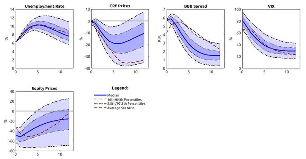
Notes: The solid line represents the point estimate (median) of the impulse response distribution. The dotted lines represent the 16th and 84th percentiles of the posterior distribution, with the darker shaded region pointwise containing 68 percent of the probability mass. The dash-dotted lines represent the 2.5th and 97.5th percentiles of the posterior distribution, with the lighter shaded region pointwise containing 95 percent of the probability mass. The dashed line represents the average scenario path for each variable across severely adverse scenarios from 2014-2025. Stock prices and commercial real estate (CRE) prices enter the estimation in log levels; all other variables enter the estimation in levels. The BBB spread is defined as the quarterly average of daily ICE BofAML U.S. Corporate 7-10 Year Yield-to-Maturity Index relative to the quarterly average of daily 10-year Treasury yields.
Sources: U.S. unemployment rate: Quarterly average of seasonally adjusted monthly unemployment rates for the civilian, non-institutional population aged 16 years and older, Bureau of Labor Statistics (series LNS14000000); U.S. Commercial Real Estate Price Index: Commercial Real Estate Price Index, Z.1 Release (Financial Accounts of the United States), Federal Reserve Board (series FL075035503.Q divided by 1000); U.S. BBB corporate yield: Quarterly average of daily ICE BofAML U.S. Corporate 7-10 Year Yield-to-Maturity Index, ICE Data Indices, LLC, used with permission (C4A4 series); U.S. 10-year Treasury yield: Quarterly average of the daily yield on 10-year U.S. Treasury notes, constructed by Federal Reserve staff based on the Svensson smoothed term structure model (see Lars E. O. Svensson, 1995, “Estimating Forward Interest Rates with the Extended Nelson–Siegel Method,” Quarterly Review, no. 3, Sveriges Riksbank, pp. 13–26); U.S. Market Volatility Index (VIX): VIX converted to quarterly frequency using the maximum close-of-day value in any quarter, Chicago Board Options Exchange via Bloomberg Finance L.P; U.S. Dow Jones Total Stock Market (Float Cap) Index: End-of-quarter value via Bloomberg Finance L.P.
The BBB spread response is displayed in the third panel of the top row of Figure 2. The size of the shock is chosen such that the implied peak would be quantitatively close to the peak values observed during the 2007-2009 financial crisis – about 6 percentage points, as discussed in the previous section. BBB spread increases on impact and reaches a peak of about 5.9 percentage points in quarter two. Given that the BBB spread was on average 1.8 percentage points over the estimation sample, the increase implies about a 4.1 percentage point increase from this initial condition at the median. Taking estimation uncertainty into account, the darker-shaded band region around this median estimate would imply that the median peak lies in the interval of 5.5 to 6.2 percentage points. Accordingly, this interval is rather tight and encompasses the historical observation of about 6 percentage points. Additionally, the VAR-implied peak occurs early on, in the second quarter, which is also very similar to the timing of the peak observed in the 2007-2009 financial crisis. The scenario-implied peak is located within the shaded region as well. After the peak, the median trajectory implied by the impulse response resembles the pattern in the historical data during the 2007-2009 financial crisis rather well. Post-peak average scenario trajectory is outside of the narrower darker-shaded band region but mostly inside the lighter-shaded band region. Also, the scenario-implied end point of the trajectory is located well within the lighter-shaded region, at the margin of the darker-shaded region.
The rest of the variables in the model are ordered such that the unemployment rate and CRE prices do not respond to the shock on impact, while the VIX and equity prices are able to respond on impact. This assumption reflects the fast-moving nature of equity prices and VIX, and the slower moving nature of the unemployment rate and CRE prices. We consider this ordering as our baseline specification and later relax this assumption, when testing the robustness of the baseline results.
The top left panel of Figure 2 shows the response of the unemployment rate to the shock in the BBB spread. At its peak, the unemployment rate increases by about 4 percentage points from the baseline (sample average). This peak is achieved in the sixth quarter of the horizon. Given that the unemployment rate is on average about 6 percent over the estimation sample, this implies a peak unemployment rate of about 10.3 percent in response to the shock. Both the magnitude of the response and its timing are similar to the 2007-2009 financial crisis data and very close to the typical past average scenario trajectories for the unemployment rate. In fact, the typical scenario trajectory almost overlaps with the median estimate for the entire horizon.
The second panel in the top row of Figure 2 shows the response of CRE prices to the BBB spread shock. CRE prices steadily decline following the shock and reach a trough that is about 20 percent lower than the jump-off value. In the previous section, we documented that the corresponding decline during the 2007-2009 financial crisis, as well as in a typical scenario, amounted to about 35 percent, which is larger than the median impulse response but still encompassed by the bands of lighter-shaded region. This result of a somewhat less pronounced median response at the trough appears intuitive, since by design the threshold-VAR methodology averages across episodes of largely business-cycle frequency, when volatility, spreads and unemployment surge, while equity prices fall. CRE cycles are known to be longer than business cycles, hence such averaging is likely to dampen the CRE results disproportionately more. Additionally, the trough of the CRE price impulse occurs 7 quarters after the shock, suggesting a slower moving price decline, which is broadly consistent with both the historical experience of the 2007-2009 financial crisis (trough at quarter 6) as well as a typical stress test scenario (trough at quarter 8).
The fourth panel on the top row of Figure 2 shows the response of the imputed equity price volatility measure. The imputed measure of volatility has a different standard deviation than the VIX. Therefore, to compare these results to the historical experience (based on the VIX), we need to account for this difference in scaling. On impact, this variable reaches its peak value of 81 percent, with the darker-shaded bands encompassing values of 74 to 89 percent. Recall that VIX reached a peak of about 80 during the 2007-2009 financial crisis, as described in the previous section. Hence, after proper rescaling, the results based on the imputed volatility measure are quantitatively consistent with this historical evidence. Furthermore, the peak value of the volatility measure occurs on impact, followed by a gradual decline over the considered horizon, also closely resembling the features documented earlier. In fact, the scenario-implied trajectory is almost entirely contained within the darker-shaded bands, except for the impact period, when it is contained within the lighter-shaded bands. This impulse response is supportive of a fast-moving volatility reaction to the shock and its subsequent gradual decline. Similar to the BBB spread, the post-peak median trajectory is largely close to the historical time series of the VIX during the 2007-2009 financial crisis, although the historical time series is somewhat more volatile in the second half of the trajectory.
Lastly, the only chart on the second row of Figure 2 shows the response of equity prices to the BBB spread shock. Equity prices fall sharply on impact and reach a trough in the second quarter, followed by a gradual return to the baseline. At the trough, median response indicates that equity prices fall 52 percent relative to the jump-off. The 16- to 84-percentile bands (darker-shaded region) imply a trough equity price decline ranging from 43 to 62 percent. These magnitudes are very similar to the historical experience documented earlier, as well as the typical trough decline in the past stress test scenarios. Additionally, the trough of the equity price decline occurs 2 quarters after the shock, suggesting a fast-moving, front-loaded price decline, a quarter faster than during the 2007-2008 financial crisis and two quarters faster than a typical stress test scenario would imply. The overall trajectory implied by the impulse response is rather close to the trajectory observed during the 2007-2009 financial crisis. The scenario trajectory is almost entirely encompassed by the darker-shaded band region; the only point outside of it is in the impact period and is covered by the lighter-shaded band region.
Taken together, the impulse response results in this VAR exercise provide further evidence that the comovement of key domestic scenario variables, i.e., direction of change, magnitudes of change, manner of change and its timing, are reasonable and find substantial empirical support in the data.
VAR Robustness
The results of the VAR exercise are robust to several implementation choices. First, the results are strongly robust to the choice of a different lag order in the system. In particular, lag orders between two and nine deliver nearly identical results.
Second, an important assumption in the shock identification is the ordering of variables. Although ordering the unemployment rate first is consistent with the macroeconomic literature (see, for example, Gilchrist and Zakrajsek (2012)), we explore alternative plausible orderings. The results are qualitatively similar when we allow the unemployment rate and CRE prices to respond on impact as well. In the case of CRE prices, the impact response turns out to be close to zero and statistically insignificant. The response of unemployment on impact is statistically significant, yet quantitatively small, measuring about 0.3 percentage points above the initial condition for the median estimate. Accordingly, allowing these variables to respond on impact does not substantially alter the key qualitative and quantitative characteristics of the impulse responses, as their shape, peak or trough magnitude and their corresponding timing remain very similar to the baseline results. The order of variables, when unemployment can respond on impact, is well aligned with the narrative of the stress test scenario that would postulate an increase in the unemployment rate along with a financial shock early in the scenario. Therefore, robustness to this specification is particularly reassuring.
Third, the results are robust to using alternative measures for equity volatility and the corporate spread.16 Substituting the imputed equity volatility measure for the VIX series limits the start of the sample to 1990Q1. For comparability with the baseline estimation, the sample in this robustness exercise also ends in 2019Q4.17 Given a substantially smaller sample size relative to our baseline exercise, we estimate the VAR on this full sample without isolating the stressful episodes with a TVAR approach.18 The results from this exercise are shown in Figure 3.
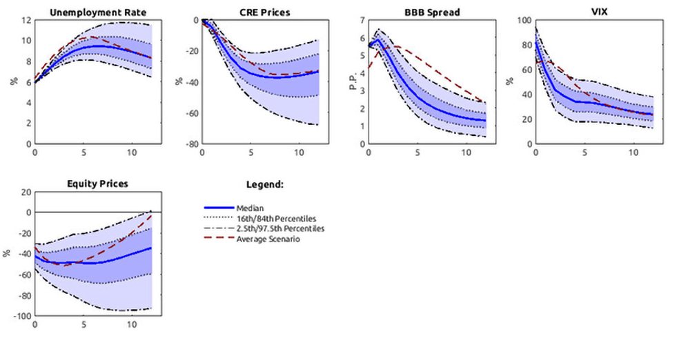
Notes: The solid line represents the point estimate (median) of the impulse response distribution. The dotted lines represent the 16th and 84th percentiles of the posterior distribution, with the darker shaded region pointwise containing 68 percent of the probability mass. The dash-dotted lines represent the 2.5th and 97.5th percentiles of the posterior distribution, with the lighter shaded region pointwise containing 95 percent of the probability mass. The dashed line represents the average scenario path for each variable across severely adverse scenarios from 2014-2025. Stock prices and commercial real estate (CRE) prices enter the estimation in log levels; all other variables enter the estimation in levels. The BBB spread is defined as the quarterly average of daily ICE BofAML U.S. Corporate 7-10 Year Yield-to-Maturity Index relative to the quarterly average of daily 10-year Treasury yields.
Sources: U.S. unemployment rate: Quarterly average of seasonally adjusted monthly unemployment rates for the civilian, non-institutional population aged 16 years and older, Bureau of Labor Statistics (series LNS14000000); U.S. Commercial Real Estate Price Index: Commercial Real Estate Price Index, Z.1 Release (Financial Accounts of the United States), Federal Reserve Board (series FL075035503.Q divided by 1000); U.S. BBB corporate yield: Quarterly average of daily ICE BofAML U.S. Corporate 7-10 Year Yield-to-Maturity Index, ICE Data Indices, LLC, used with permission (C4A4 series); U.S. 10-year Treasury yield: Quarterly average of the daily yield on 10-year U.S. Treasury notes, constructed by Federal Reserve staff based on the Svensson smoothed term structure model (see Lars E. O. Svensson, 1995, "Estimating Forward Interest Rates with the Extended Nelson–Siegel Method," Quarterly Review, no. 3, Sveriges Riksbank, pp. 13–26); U.S. Market Volatility Index (VIX): VIX converted to quarterly frequency using the maximum close-of-day value in any quarter, Chicago Board Options Exchange via Bloomberg Finance L.P; U.S. Dow Jones Total Stock Market (Float Cap) Index: End-of-quarter value via Bloomberg Finance L.P.
For comparability with the earlier results, we produce the impulse responses to a BBB spread shock, targeting the same peak value response as in the baseline exercise, and find that the results overall are still rather similar. Furthermore, the shapes of the other impulse responses are also very close, with the timing of peaks and troughs remaining broadly similar or often identical (Figure 3). The response of the unemployment rate is nearly identical, with a peak timing now delayed by one quarter relative to the baseline result. The response of equity prices is similar, yielding a trough decline at the median of around 49 percent. In the case of VIX, the peak of 82 percent at the median is very similar to the baseline exercise, after taking into account the corresponding initial condition.19 As for CRE, the trough at the median now measures about 37 percent deviation from the baseline (compared with about 20 percent in the TVAR specification) - a substantially more pronounced decline. This result matches the average trough in past scenarios and in the 2007-2009 financial crisis rather well, better than the TVAR specification. The reason why the response of the CRE prices in particular is more magnified in this case is related to the sample. Unlike in the TVAR exercise, where some of the selected stress episodes by construction could not adequately reflect the slower-moving CRE price cycle, picking up only some parts, the smaller sample of this exercise being centered around the 2007-2009 financial crisis did just that, which resulted in a more pronounced quantitative effect.
As an additional robustness check, we also compared our baseline findings with the results in the literature. In doing so, we focused on identification strategies with no a-priori directional assumptions on the variables and studies of VAR systems containing variables similar to ours. The identification strategy employed by Angeletos et al. (2020) satisfies these criteria. They explore a system of U.S. variables that (among other variables) contains the unemployment rate, GDP growth and corporate spreads. Adjusted for the same shock size, the comovement between real variables and the corporate spreads is broadly consistent with our baseline findings.20 Hence, also from a perspective of a completely different shock identification and estimation strategy, the scenario-implied comovement between real variables in corporate spreads appears reasonable.
Conclusion
This note applies several tools to investigate the empirical regularities in the comovement of key domestic variables in Federal Reserve's stress test scenarios. Our comprehensive analysis, using both historical comparisons and VAR modeling, provides strong evidence that the comovement patterns of macroeconomic variables in the Board's stress tests are well-grounded in empirical data, both qualitatively and quantitatively. This lends credibility to the design of the stress test scenarios and reinforces their validity as tools for assessing bank resilience.
References
Aikman, D., A. Lehnert, N. Liang and M. Modugno (2020). "Credit, Financial Conditions, and Monetary Policy Transmission." International Journal of Central Banking 16(3): 141-179.
Angeletos, G.-M., F. Collard, H. Dellas (2020). "Business-Cycle Anatomy." American Economic Review, 110(10): 3030-70.
Antolin-Diaz, J. and J. F. Rubio-Ramirez (2018). "Narrative Sign Restrictions." American Economic Review, 108(10): 2802-29.
Ariaz, J.E., J. F. Rubio-Ramirez and D. F. Waggoner (2018). "Inference Based on Structural Vector Autoregressions Identified with Sign and Zero Restrictions: Theory and Applications." Econometrica 86(2): 685-720.
Caldara, D. and E. Herbst (2019). "Monetary Policy, Real Activity, and Credit Spreads: Evidence from Bayesian Proxy SVARs." Americal Economic Journal: Macroeconomics 11(1): 157-192.
Giannone, D., Lenza, M., and Primiceri, G. E. (2015). "Prior Selection for Vector Autoregressions." The Review of Economics and Statistics, 97(2), 436–451.
Gilchrist, S., Zakrajsek, E. (2012). "Credit Spreads and Business cycle Fluctuations." American Economic Review, 102(4), 1692-1720.
Krishnamurthy, A. and K. Li (2025). "Dissecting Mechanisms of Financial Crises: Intermediation and Sentiment." Journal of Political Economy 133(3): 935-985.
Lenza, M. and G. Primiceri (2022). "How to Estimate a Vector Autoregression after March 2020." Journal of Applied Econometrics 37: 688-699.
Litterman, R. (1980). "A Bayesian Procedure for Forecasting with Vector Autoregression." Working Paper, MIT, Department of Economics.
Wiggins, R. Z., T. Piontek and A. Metrick (2019). "The Lehman Brothers Bankruptcy A: Overview". Journal of Financial Crises 1(1): 39-62.
Appendix
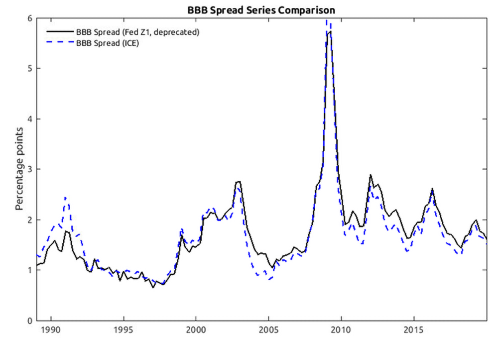
Notes: Yield on BBB corporate bonds data for the BBB Spread (Fed Z1, deprecated) measure are the Merrill Lynch 10-year BBB corporate bond yield, Z.1 Release (Financial Accounts of the United States), Federal Reserve Board (series FL073163013.Q) which is no longer published; Yield on BBB corporate bonds data for the BBB Spread (ICE) measure are the quarterly average of daily ICE BofAML U.S. Corporate 7-10 Year Yield-to-Maturity Index, ICE Data Indices, LLC, used with permission (C4A4 series); 10-year Treasury yield data are constructed by Federal Reserve staff based on the Svensson smoothed term structure model (see Lars E. O. Svensson, 1995, "Estimating Forward Interest Rates with the Extended Nelson–Siegel Method," Quarterly Review, no. 3, Sveriges Riksbank, pp. 13–26).
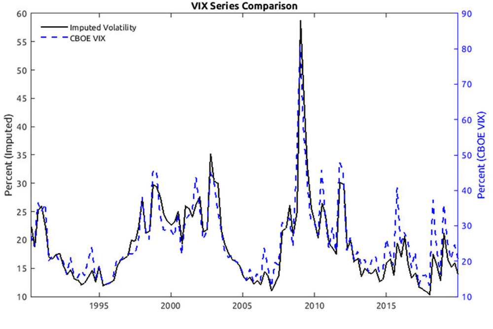
Notes: Imputed Volatility measure is computed on S&P 500 Composite data from Bloomberg Finance LP; CBOE VIX data are from Chicago Board Options Exchange via Bloomberg Finance L.P.
1. We thank Michele Modugno and Molin Zhong for helpful comments and discussions. The note reflects the views of the authors and should not be interpreted as reflecting the views of the Board of Governors of the Federal Reserve System or anyone else associated with the Federal Reserve System. Return to text
2. Board of Governors of the Federal Reserve System. (2025). "2025 Stress Test Scenarios". Return to text
3. These variables include nominal and real GDP, disposable income, unemployment rate, inflation, Treasury rates (3-month Treasury rate, 5-year and 10-year Treasury yields), mortgage spread, BBB spread, VIX, equity prices, commercial real estate (CRE) prices, and housing prices. Return to text
4. For the specific variable definitions and construction, see the notes to Figure 2. Return to text
5. For more information about the Federal Reserve's framework for designing stress test scenarios, see "Policy Statement on the Scenario Design Framework for Stress Testing" (12 CFR part 252, appendix A). Return to text
6. Id., at section 4.2.1. Return to text
7. In the case of trending variables (such as asset prices), indexing is applied to ensure comparability. In particular, the series in each scenario and in the historical data are rescaled, such that the starting point would amount to 100 percent. The jump-off points (or initial conditions), from which the scenario trajectory starts, are also taken from the published scenarios. Return to text
8. See, for example, Wiggins et al. (2019). Return to text
9. For more details see: Federal Reserve Board - Treasury and Federal Reserve announce launch of Term Asset-Backed Securities Loan Facility (TALF). Return to text
10. See, for example, the Federal Reserve Board's scenario disclosures available online here: The Fed - Dodd-Frank Act Stress Test Publications. Return to text
11. For the baseline exercise, we use the S&P 500 Composite Index rather than the Dow Jones Price Index Series for our measure of equity prices as the former has a longer sample available. The two series have a correlation of over 99 percent from 1990Q1-2019Q4 and, as discussed in the robustness section, using one or the other in this setting does not alter the results. Return to text
12. This version of the BBB spread uses a different measure for the BBB corporate yield. This measure is 'Merrill Lynch 10-year BBB corporate bond yield', which was previously published in the Federal Reserve Board's Financial Accounts of the United States (Z.1 Release, series FL073163013.Q). The imputed measure of volatility is constructed as follows. We first construct a measure of volatility based on daily S&P 500 returns and then aggregate it to monthly frequency by averaging. We then compute the ratio of actual VIX to this series over the overlapping sample, compute the average ratio, and scale this series by that scaling factor. As a final step, we convert the resulting measure to quarterly frequency by taking the average. Return to text
13. As is common in this literature, Giannone et al. (2015) rely on the Minnesota prior introduced and popularized by Litterman (1980). We follow Giannone et al. (2015) in the method of calibrating this prior, i.e., choosing its hyperparameters. Return to text
14. The stressful periods used in the threshold VAR analysis include 1972Q1-1975Q4, 1980Q1-1984Q4, 1988Q1-1991Q4, 2000Q1-2002Q4, and 2007Q1-2011Q4. These periods were chosen based on the behavior of the variables in the system, with most variables moving in the direction of indicative of stress during each period. These periods turn out to be similar to the dates of NBER-defined recessions. Return to text
15. They consider shocks to the excess bond premium – the component of corporate spreads that is orthogonal to firm-specific information on expected defaults. Return to text
16. Relatedly, the results are nearly identical when we use the Dow Jones index instead of the S&P 500 index on conformable samples. Return to text
17. It is well documented in the literature that the inclusion of COVID can affect estimation of the VARs and therefore their forecasting qualities and sometimes also impulse responses (see Lenza and Primiceri, 2022, for example). In our case, stopping the sample in 2024 Q3 (i.e., including the COVID pandemic) produces overall rather similar impulse responses. One notable exception is the impulse response of the unemployment rate, which implies a steeper increase trajectory to the peak, yet a very similar peak magnitude and similar overall persistence of the impulse response. Return to text
18. The lag order in this robustness exercise is set to 5 quarters, as in the baseline TVAR specification. Similar to the TVAR specification, the results here are robust to lag order variations from 2 to 9. Return to text
19. For internal consistency, the typical initial condition in this case corresponds to the average of VIX across the estimation sample – 1990 Q1 through 2019 Q4. Return to text
20. The authors report a one-standard deviation shock, which is different from the shock size we are interested in. Hence, we rescaled the shock and the implied response accordingly. If we adjust the size of their shock such that their reported peak unemployment rate response lines up with our calibration (increase from the sample average by 6 p.p. to achieve a level of 10 percent) and recompute the peak response of the corporate spread, we would get an increase in the spread by about 8 p.p., which is more severe than the 6 percentage point peak observed during the 2007-2009 financial crisis. A similar result obtains, if we instead target the authors' response of GDP growth, rescale it and recompute the corporate spread response. Return to text
Afanasyeva, Elena, William F. Bassett, Bora Durdu, Sam Jerow, and Fiona C. Waterman (2025). "Evaluating Empirical Regularities in Variable Comovement in Stress Test Scenarios," FEDS Notes. Washington: Board of Governors of the Federal Reserve System, September 19. 2025, https://doi.org/10.17016/2380-7172.3885.
Disclaimer: FEDS Notes are articles in which Board staff offer their own views and present analysis on a range of topics in economics and finance. These articles are shorter and less technically oriented than FEDS Working Papers and IFDP papers.