FEDS Notes
November 17, 2022
House Price Growth and Inflation During COVID-191
Aditya Aladangady, Elliot Anenberg, and Daniel Garcia
1. Introduction
House prices have risen rapidly during the pandemic, creating $9 trillion in owner occupied housing wealth between the first quarter of 2020 and the first quarter of 2022. Both housing and non-housing inflation also moved up over this time period to its highest level in many decades. This note considers whether the large increase in housing wealth has been an important contributor to non-housing inflation during the pandemic.
There are two main channels through which increases in housing wealth can contribute to non-housing inflation. First, the increase in housing wealth can stimulate additional consumption among existing homeowners, either because they feel wealthier or by relaxing borrowing constraints (Guren et al., 2021; Mian, Rao and Sufi, 2013; Aladangady, 2017). This shift in aggregate demand can result in non-housing inflation, especially when the slope of the aggregate supply curve is steep, as may have been the case during the pandemic. Second, homeowners may become less price sensitive as they become wealthier, allowing some firms to respond to a less price-elastic demand curve by raising markups and prices (Stroebel and Vavra, 2019).
This note documents a strong positive association between non-housing inflation and house price growth across major metropolitan areas during the first two years of the pandemic. Also, we show this correlation is much stronger than in recent history. The association during the pandemic does not appear to be driven by other leading omitted variables that could be correlated with local house price growth and inflation, such as changes in the local unemployment rate or population growth. In addition, we find a strong cross-sectional correlation between house price growth and both nominal and real credit card spending.
Taken together, our results provide suggestive evidence that house price growth has been an important contributor to inflation during the pandemic, in part by shifting aggregate demand along a steeper-than-normal aggregate supply curve. A back-of-the-envelope calculation based on our regression estimates suggests that house price growth could explain about 1/3 of the increase in the consumer price index (CPI) excluding housing services between February 2020 and February 2022. At the lower bound of the 90 percent confidence interval around our regression estimate, house price growth still explains 13 percent of the increase in the CPI excluding housing services.
2. Inflation and House Price Growth Across Metro Areas
We estimate the cross-sectional relationship between inflation and house price growth using the regression equation:
$$(1) \ \ \ \ \ \Delta log({cpix}_i) = \beta_0 + \beta_1 \Delta log({hpi_i}) + \beta_2 X_i + \varepsilon_i $$
where $$cpix$$ is the CPI excluding housing services for metro area $$i$$, $$hpi$$ is the CoreLogic house price index for metro area $$i$$, $$X_i$$ is a vector of other local characteristics, and $$\Delta$$ denotes the two-year change in the variable, February 2022 relative to February 2020.
The CPI is available for the 21 largest metro areas in the country, in addition to Honolulu, HI and Anchorage, AK, which jointly account for about 40 percent of the U.S. population. Table 1 reports summary statistics and sources for the variables used in this analysis.
Table 1: Summary Statistics
| count | mean | sd | min | max | |
|---|---|---|---|---|---|
| Inflation | 23 | 0.1090511 | 0.0170322 | 0.0846398 | 0.1463565 |
| House Price Growth | 23 | 0.2491956 | 0.0771626 | 0.1483944 | 0.4208717 |
| Spending Growth | 23 | 0.1335134 | 0.0494398 | 0.0287648 | 0.2199959 |
| Population Growth | 23 | -0.0061354 | 0.0154132 | -0.0340388 | 0.0279839 |
| U rate Change | 23 | 0.6478099 | 0.740321 | -1.14869 | 1.699577 |
| Personal Inc. Growth, 2019-2020 | 23 | 0.061984 | 0.0203732 | 0.0171909 | 0.1070625 |
| Average Dividend + Interest Inc., 2019 | 23 | 5360.437 | 2240.583 | 1371.291 | 10421 |
| College Share 2015-2019 | 23 | 0.3750992 | 0.0685322 | 0.2169467 | 0.5094283 |
| Median Income 2015-2019 | 23 | 75838.39 | 13257.17 | 55285 | 106025 |
| Homeownership Rate 2015-2019 | 23 | 0.6167216 | 0.0571127 | 0.4856795 | 0.6995842 |
| Median Age 2015-2019 | 23 | 37.48696 | 2.090303 | 34 | 42.1 |
| Market Rent Growth | 21 | 0.1449186 | 0.0885461 | 0.0057963 | 0.3616535 |
Notes: Inflation is difference in the log CPI less shelter price index between February 2020 and February 2022. House price growth is the difference in log CoreLogic house price between 2020Q1 to 2022Q1. Spending is the difference in log new credit card spending between January-February 2020 and January-February 2022 calculated using the Y14 data. Population growth is the net migration rate between February 2020 and February 2022, calculated using the FRBNY/Equifax Consumer Credit Panel, following the definition in Mondragon and Wieland (2022). Change in unemployment rate is percentage point change between February 2020 and February 2022 from BLS. Personal income growth is from the Bureau of Economic Analysis (BEA). Per capita interest and dividend income is from the 2019 Internal Revenue Service’s Statistics of Income (IRS SOI). Demographics come from the 2015-2019 Census Bureau’s American Community Survey (ACS). Market rate rent growth is log difference in the CoreLogic single-family rent index between February 2020 and February 2022.
The scatter plot in Figure 1 shows a strong positive association between $$\Delta log({cpix}_i)$$ and $$\Delta log({hpi_i})$$. Table 2, column 1 shows that a one percentage point increase in house price growth is associated with a 0.15 percentage point increase in inflation. Also, house price growth alone explains 42 percent of the cross-sectional variation in non-housing inflation during the pandemic.
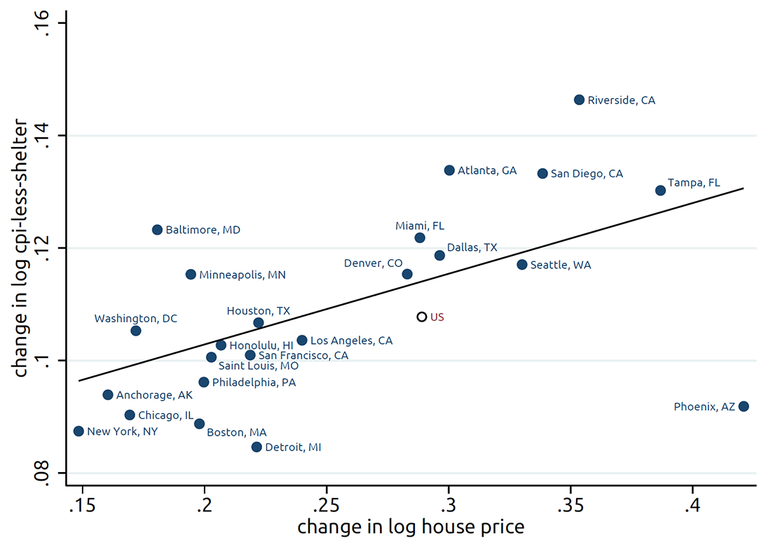
Notes: Trend line estimated excluding the observation for the United States.
Table 2: House Price Growth and CPI-less-shelter Growth by CBSA, February 2020-February 2022
| Inflation | Inflation | Inflation | Inflation | Inflation | Inflation | Inflation | Inflation | |
|---|---|---|---|---|---|---|---|---|
| House Price Growth | 0.145∗∗ | 0.119∗ | 0.147∗∗∗ | 0.149∗∗ | 0.136∗∗ | 0.136∗ | 0.188∗∗ | 0.127∗ |
| (0.0597) | (0.0678) | (0.0495) | (0.0577) | (0.0602) | (0.0683) | (0.0824) | (0.0697) | |
| Population Growth | 0.163 | -0.265 | ||||||
| (0.1530) | (0.5770) | |||||||
| U rate Change | 0.452 | 0.607 | ||||||
| (7.0300) | (10.0200) | |||||||
| Personal Inc. Growth, 2019-2020 | -0.11 | -0.27 | ||||||
| (0.1390) | (0.3940) | |||||||
| Average Dividend + Interest Inc., 2019 | -0.0985 | -0.179 | ||||||
| (0.1370) | (0.2270) | |||||||
| College Share 2015-2019 | -0.0277 | -0.058 | ||||||
| (0.1310) | (0.2040) | |||||||
| Median Income 2015-2019 | 0.00189 | 0.00447 | ||||||
| (0.0059) | (0.0094) | |||||||
| Homeownership Rate 2015-2019 | 0.0278 | 0.00993 | ||||||
| (0.0336) | (0.0633) | |||||||
| Median Age 2015-2019 | -0.139 | 0.011 | ||||||
| (0.1520) | (0.2800) | |||||||
| Market Rent Growth | 0.0229 | |||||||
| (0.0249) | ||||||||
| R-Squared | 0.423 | 0.432 | 0.423 | 0.437 | 0.436 | 0.463 | 0.484 | 0.424 |
| N | 23 | 23 | 23 | 23 | 23 | 23 | 23 | 21 |
Standard errors in parentheses
∗ p < 0.1, ∗∗ p < 0.05, ∗∗∗ p < 0.01
Notes: Robust standard errors are reported. Observations are weighted by the size of the housing stock. Some variables reported in Table 1 are rescaled for the regression results for ease of presentation. Change in unemployment rate is percentage point change divided by 1,000. Per capita interest and dividend income is divided by 100,000. Median age is divided by 100 and median household income is divided by 10,000.
The remaining columns in Table 2 add various controls, $$X_i$$, to address leading potential omitted variables. One possibility is that areas with high house price growth saw increases in population during the pandemic, and the increase in population increased aggregate demand and inflation. Even though there is a strong relationship between population and house price growth during the pandemic, the results in column 2 show that the estimated elasticity of non-housing inflation to house price growth is little changed when adding population growth as a control.
Another possibility is that house price growth is associated with the strength of the local labor market, and it is local labor market conditions that influence inflation, not house price growth directly. The results in column 3, however, show that the estimated elasticity of non-housing inflation to house price growth is little changed when adding the change in the unemployment rate as a control.2 Also, the coefficient on house price growth is similar when controlling for the growth in average weekly wage changes or the total wage bill from the Quarterly Census of Employment and Wages (not shown).
Over our sample period, Congress passed massive fiscal stimulus, and the generosity of the income support from these stimulus programs likely varied across metro areas. It is possible that local income growth drove both house price growth and inflation. In column 4, we control for the growth in personal income as measured by the BEA, which includes income that people get from government benefits.3 Personal income growth is not significantly associated with inflation, and again the estimated elasticity of inflation to house price growth is little changed when adding local income growth as a control. Next, we consider the possibility that the housing wealth effect on inflation that we estimate may be correlated with a stock market wealth effect. Like house prices, stock prices soared in 2020 and 2021. We proxy for local exposure to increases in stock market wealth with the per-capita pre-pandemic average interest and dividend income in the metro area calculated from the 2019 IRS SOI tax data. Column 5 shows the results are little changed when this variable is added as a control. Column 6 shows results with controls for pre-pandemic median household income, share of households with college education, the homeownership rate, and median age – potential alternative proxies for exposure to the stock market boom. The results are similar.
Column 7 shows the results when all controls are added. None of the controls are individually significant, and the estimated elasticity of inflation to house price growth remains sizable and significant. Finally, column 8 includes as a control the log change in market-rate rents, available for 21 of the metro areas in our sample. The coefficient on house price growth remains of a similar magnitude as in other specifications and remains significant. This is further evidence that the coefficient on house price growth is primarily measuring housing wealth effects rather than confounding factors, as changes in market rate rents should reflect various unobserved factors associated with housing demand and supply that could be correlated with house price growth and inflation. Indeed, changes in rents are highly correlated with changes in house prices, inflation, and population.
In sum, looking across all the columns in the table, the estimated elasticity is remarkably stable considering the small sample size. A natural question is what is driving the variation in house prices across cities. While pinpointing the causes of house price changes is beyond the scope of this Note, some factors that could drive cross-sectional variation in house price growth that are plausibly unrelated to inflation include housing supply elasticity, the increase in demand for second homes from out-of-town buyers, or the pre-pandemic work-from-home share (Mondragon and Wieland, 2022). We explore instruments for house price growth in future work.
2.1. Inflation by type of goods or services
Table 3 shows results separately for inflation of durable goods, nondurable goods, services excluding shelter, and shelter services. We find the strongest effects of house price growth on inflation for services excluding shelter, nondurable goods and shelter services. For durable goods, we estimate a small or very noisy effect of house price growth on inflation. House price growth may not have a clear effect on durable goods inflation because durable goods are less likely to be produced locally (e.g. motor vehicles), and therefore, firms selling durable goods may set prices nationally. It is possible that house price growth increases inflation for durable goods, but trade reduces differences across metro areas. Our cross-sectional estimation strategy cannot identify this type of aggregate effect.
Table 3: House Price Growth and CPI growth by Type of CPI Good or Service, February 2020 - February 2022
| Serv. ex shelter | Durables | NonDurables | Shelter | Serv. ex shelter | Durables | NonDurables | Shelter | |
|---|---|---|---|---|---|---|---|---|
| House Price Growth | 0.177∗∗ | -0.0742 | 0.138∗∗ | 0.344∗∗∗ | 0.294∗∗ | -0.437∗ | 0.212∗∗ | 0.259∗∗ |
| (0.0728) | (0.0915) | (0.0546) | (0.0678) | (0.1170) | (0.2230) | (0.0879) | (0.0941) | |
| Controls | N | N | N | N | Y | Y | Y | Y |
| R-squared | 0.357 | 0.0222 | 0.327 | 0.631 | 0.531 | 0.324 | 0.516 | 0.92 |
| N | 23 | 23 | 23 | 23 | 23 | 23 | 23 | 23 |
Standard errors in parentheses
∗ p < 0.1, ∗∗ p < 0.05, ∗∗∗ p < 0.01
Notes: Robust standard errors are reported. Observations are weighted by the size of the housing stock. For specifications that include controls, the controls are those listed in column 7 of Table 2.
The very strong effect of house price growth on shelter services inflation shown in columns 4 and 8 is unlikely to be entirely causal. There is no mechanical link between the two, as shelter services inflation is based on rents for renters and a measure of implied rents for owners.4 That said, when housing supply is constrained, a positive housing demand shock will tend to raise both house prices and rents, leading to a positive correlation between house price growth and shelter services inflation. For this reason, we remove shelter inflation from the measure of inflation we use for the results in Table 2. Still, there is potential for some causal effect of house price growth on shelter inflation as discussed in Dias and Duarte (2019).
2.2. Comparing the pandemic inflation-house price growth relationship with its historical one
An increase in non-housing demand, induced by increases in housing wealth, is likely to be more inflationary when supply is more constrained. Since the second half of 2020 through the start of 2022, supply conditions have seemed generally tight, with retailers reporting low inventories and producers reporting slow delivery times amid shortages of inputs used in production. Hence, our prior is that demand effects were likely more inflationary from February 2020 to February 2022 than in other periods.
Table 4 shows results from a regression of non-shelter inflation on house price growth using metro area observations pooled across all two-year periods between February 2000 and February 2022. The regression includes an interaction between house price growth and a dummy variable for the 2020 to 2022 pandemic period allowing us to estimate the relation between house prices and inflation separately in the pre-pandemic and pandemic periods. The results in column 2 include metro area fixed effects and the results in column 3 include both metro area fixed effects and time period fixed effects. The results across all three columns show that the association between inflation and house price growth was unusually strong during the pandemic. Indeed, in the two decades prior to the pandemic, there was essentially no correlation between house price growth and non-shelter inflation for these metropolitan areas.
Table 4: House Price Growth and CPI-less-shelter Growth by CBSA, Nonoverlapping 2-year periods from February 2000 - February 2022
| (1) Inflation |
(2) Inflation |
(3) Inflation |
|
|---|---|---|---|
| House Price Growth | 0.00168 | 0.000548 | -0.00271 |
| (0.00975) | (0.0102) | (0.00798) | |
| House Price Growth * Pandemic Dummy | 0.274∗∗∗ | 0.276∗∗∗ | 0.127∗∗∗ |
| (0.0213) | (0.0225) | (0.0300) | |
| CBSA FE | No | Yes | Yes |
| 2-year Time Period FE | No | No | Yes |
| R-squared | 0.371 | 0.383 | 0.902 |
| N | 318 | 318 | 318 |
Standard errors in parentheses
∗ p < 0.1, ∗∗ p < 0.05, ∗∗∗ p < 0.01
Notes: The metro areas with available inflation data varies somewhat over time. In the early 2000s, the BLS inflation data exists for 28 metro areas; during the pandemic period, it exists for only 23 metro areas. Observations are weighted by the size of the housing stock. Pandemic dummy is a dummy variable for the period February 2020 - February 2022.
3. Spending and House Price Growth Across Metro Areas
The main mechanism through which house prices would affect non-shelter inflation is through shifts in demand or changes in markups arising from housing wealth effects. To provide evidence consistent with these mechanisms, we use data on credit card spending from the Federal Reserve Board's FR Y-14M reports. These reports require large U.S. bank holding companies, with at least $100 billion in total assets, to report information on individual credit card accounts on a monthly basis. For each metro area, we construct the change in nominal spending as measured by the flow of new purchases on credit cards between January-February 2020 and January-February 2022.5 For the 23 metro areas for which we observe CPI, we also construct a change in real spending by deflating nominal spending with the local CPI less shelter over the same time period.
Table 5 shows results of regressions similar to equation 1, replacing the dependent variable with spending growth. The first column shows that the estimated nominal spending elasticity to house price growth is 0.58 for the same small sample of metro areas used in Table 2. Column 2 shows the elasticity is little changed when the controls are added to the regression. The third and fourth columns show the real spending elasticity is strongly positive but smaller than the nominal elasticity, consistent with the positive association between inflation and house price growth shown in Table 2.
Table 5: House Price Growth and Credit Card Spending Growth, February 2020 -February 2022
| Nominal | Nominal | Real | Real | Nominal | Nominal | |
|---|---|---|---|---|---|---|
| House Price Growth | 0.584∗∗∗ | 0.494∗∗∗ | 0.439∗∗∗ | 0.306∗∗∗ | 0.563∗∗∗ | 0.331∗∗∗ |
| (0.0655) | (0.1170) | (0.0519) | (0.0807) | (0.0564) | (0.0398) | |
| Controls | N | Y | N | Y | N | Y |
| R-squared | 0.726 | 0.941 | 0.623 | 0.94 | 0.523 | 0.785 |
| N | 23 | 23 | 23 | 23 | 896 | 891 |
Standard errors in parentheses
∗ p < 0.1, ∗∗ p < 0.05, ∗∗∗ p < 0.01
Notes: Robust standard errors are reported for columns 1-4. Standard errors are clustered by state for columns 5 and 6. Observations are weighted by the size of the housing stock. For specifications that include controls, the controls are those listed in column 7 of Table 2. Estimates of real spending obtained by deflating nominal spending with the local CPI less shelter.
In fact, 25-40 percent of the nominal spending effect reflects an increase in prices. Focusing on spending in a sample of retail chains, Kaplan, Mitman and Violante (2020) estimated the elasticity of spending with respect to house price changes during the Great Recession. Their results suggest 20 percent of the nominal spending response during the Great Recession is due to changes in prices, with the remaining 80 percent reflecting a response in real spending.
The positive real spending response we estimate suggests a role for increased aggregate demand in explaining the positive effect of house price growth on inflation during the pandemic. Also, the substantial price response we find together with the evidence in Table 4 is consistent with tight supply conditions preventing firms from providing additional goods and services without raising prices. The price response may also be partly explained by households becoming less sensitive to price increases such that firms raised mark-ups.
Columns 5 and 6 show the elasticity of nominal spending in the full sample of 896 metropolitan and micropolitan areas covered by the Y-14M data. The estimated elasticities for the large sample are quantitatively similar to those estimated for the small sample. If we assume that 60-75 percent of the nominal spending effect in the large sample reflects an increase in real spending, consistent with the split we directly estimated for the small sample, then columns 5 and 6 imply an elasticity of non-shelter inflation with respect to house price growth of 0.125 or 0.145 for the large sample, very similar to the point estimates in Table 2 for the small sample.
4. Role of house price growth in explaining recent inflation
We can use our estimates to calculate the contribution of house price growth to national, non-shelter inflation between February 2020 and February 2022. Multiplying the increase in national house prices over this time period by the elasticity estimate from column 1 of Table 2, we find that house price growth increased the national, non-shelter CPI by 4 log points, which is 39 percent of the total increase in national, non-shelter CPI over this time period. Even at the lower bound of the 90 percent confidence interval around our elasticity estimate, house price growth still explains 13 percent of the increase in national, non-shelter CPI.
The calculation is back-of-the-envelope for a few reasons. First, it extrapolates based on a linear relationship between house price growth and inflation estimated using a sample of metro areas where house price growth was high for every observation. Still, under a very conservative scenario that assumes zero effect of house price growth on inflation until house price growth reaches the minimum level in our sample, house price growth explains 19 percent of the increase in non-shelter inflation CPI. Second, house price growth could increase price inflation for some goods or services only at the national level and not differentially by metropolitan area. Our back-of-the-envelope calculation cannot account for any national effects and thus could understate the contribution of house price growth to non-shelter inflation. Third, we cannot rule out a role for some omitted variable or measurement error to bias our estimated elasticity up or down.
Finally, the correlations we document in this note have some implications for the current inflation outlook. Following many months of annualized house price growth rates of 15-25 percent, recently house prices have decelerated sharply. The acceleration of house prices early in the pandemic preceded the acceleration in the CPI. The correlations we document in this note suggest that inflation should step down somewhat in the future, given the sharp slowdown in house price growth and absent other inflationary shocks.
References
Adams, Robert M., Vitaly M. Bord, and Bradley Katcher. 2021. "Why Did Credit Card Balances Decline so Much during the COVID-19 Pandemic?" Board of Governors of the Federal Reserve System (U.S.) FEDS Notes 2021-12-03-3.
Aladangady, Aditya. 2017. "Housing wealth and consumption: Evidence from geographically-linked microdata." American Economic Review, 107(11): 3415–46.
Dias, Daniel A, and João B Duarte. 2019. "Monetary policy, housing rents, and inflation dynamics." Journal of Applied Econometrics, 34(5): 673–687.
Guren, Adam M, Alisdair McKay, Emi Nakamura, and Jón Steinsson. 2021. "Housing wealth effects: The long view." The Review of Economic Studies, 88(2): 669–707.
Hazell, Jonathon, Juan Herreno, Emi Nakamura, and Jón Steinsson. 2022. "The slope of the Phillips Curve: evidence from US states." The Quarterly Journal of Economics, 137(3): 1299–1344.
Horvath, Akos, Benjamin S. Kay, and Carlo Wix. 2021. "The COVID-19 Shock and Consumer Credit: Evidence from Credit Card Data." Board of Governors of the Federal Reserve System (U.S.) Finance and Economics Discussion Series 2021-008.
Kaplan, Greg, Kurt Mitman, and Giovanni L. Violante. 2020. "Non-durable consumption and housing net worth in the Great Recession: Evidence from easily accessible data." Journal of Public Economics, 189: 104176.
Mian, Atif, Kamalesh Rao, and Amir Sufi. 2013. "Household balance sheets, consumption, and the economic slump." The Quarterly Journal of Economics, 128(4): 1687–1726.
Mondragon, John, and Johannes Wieland. 2022. "Housing Demand and Remote Work."
Stroebel, Johannes, and Joseph Vavra. 2019. "House prices, local demand, and retail prices." Journal of Political Economy, 127(3): 1391–1436.
1. The analysis and conclusions set forth are those of the authors and do not indicate concurrence by other members of the research staff or the Board of Governors. The authors thank Ari Gelbard, Raghav Warrier, and Adithya Raajkumar for excellent research assistance. Return to text
2. While changes in the unemployment rate are not significantly associated with inflation excluding shelter in this sample, they are negatively associated with shelter inflation. Hazell et al. (2022) find that the regional Phillips curve for rents is substantially steeper than for inflation excluding shelter. Return to text
3. Because the BEA data at a metro-area level are only available for 2020, we use personal income growth for 2020 relative to 2019. Since the progressivity of fiscal support in 2021 was similar to 2020 generally, our measure likely captures broad cross-sectional patterns in earnings and transfers over this period. Return to text
4. For more information, see https://www.bls.gov/cpi/factsheets/owners-equivalent-rent-and-rent.htm Return to text
5. Purchases on credit cards that do not become revolving balances are still included in our data. Information in the Y-14 is anonymized and does not contain transaction-level detail. Accounts associated with the same consumer cannot be linked across or within reporting banks. The large banks reporting to the FR Y-14M account for a high percentage of total credit card spending. For other work using this data, see Adams, Bord and Katcher (2021); Horvath, Kay and Wix (2021). Return to text
Aladangady, Aditya, Elliot Anenberg, and Daniel Garcia (2022). "House Price Growth and Inflation During COVID-19," FEDS Notes. Washington: Board of Governors of the Federal Reserve System, November 17, 2022, https://doi.org/10.17016/2380-7172.3228.
Disclaimer: FEDS Notes are articles in which Board staff offer their own views and present analysis on a range of topics in economics and finance. These articles are shorter and less technically oriented than FEDS Working Papers and IFDP papers.