FEDS Notes
September 19, 2025
Inflation's Shared DNA: Regional and Global Factors in Post-Pandemic Core Inflation
Daniel O. Beltran, and Julio L. Ortiz1
1. Introduction
The COVID-19 pandemic recovery created inflationary pressures globally. These effects, however, were felt differently across countries and regions. Following the sharp synchronized downturn in the first half of 2020, governments stepped in to varying degrees to stave off the unprecedented decline in economic activity. As summarized in the IMF's World Economic Outlook from April 2021:
". . . multispeed recoveries are under way in all regions and across income groups, linked to stark differences in the pace of vaccine rollout, the extent of economic policy support, and structural factors such as reliance on tourism."
The pent-up demand unleashed by the economic recovery in 2021 was followed by a rebound in commodity prices, supply disruptions and shortages, and severe dislocations in labor markets, generating inflationary pressures in both advanced and emerging market economies. Russia's invasion of Ukraine in April 2022 triggered additional increases in commodity and energy prices, and Europe's proximity to the war made it especially susceptible to energy shortages. The surge in energy and other input costs in Europe trickled down to other parts of the economy, generating persistent second-round effects to core inflation (Alp et al., 2023).
Are there meaningful regional differences in the dynamics of core inflation between Europe and North America? If so, what explains them? We address these questions using a parsimonious multivariate Bayesian time series filter that decomposes the level of core inflation in the major advanced economies into regional, global, and country-specific components. Our model is tailored to compare inflation dynamics between Europe and North America.2 The regional components are defined as the estimated levels of core inflation common to all countries in the same geographic region. The regional components may capture regional differences inflation driven by varying degrees of labor market tightness, demand conditions, monetary policy, or regional shocks such as the energy price shock in Europe following Russia's invasion of Ukraine. We identify a prominent role for regional factors, consistent with Mumtaz et al. (2011) who find that regional factors account for the bulk of fluctuations in inflation and output for most countries in their sample. Sometimes, our estimated regional components diverge, which could have implications for monetary policy. Most recently, the North American and European regional components have both largely retraced their post-pandemic increases.
After accounting for regional differences, to what extent are national core inflation rates explained by a "global" component common to all countries in our sample? Inspecting the level of our estimated global component, we find that it explains a sizable fraction of core inflation in the major advanced economies, consistent with Cascaldi-Garcia et al. (2024).3 The dynamics of our estimated global component, however, differ from prior studies due in part to the inclusion of regional components in our model. Moreover, our estimated global component seems to be driven by global supply bottlenecks (e.g., manufacturing backlogs and sea freight shipping costs) and second-round effects from past energy prices (Alp et al., 2023).
2. Data and Model Specification
Our data set is comprised of 12-month percent changes in national core consumer price indexes for 12 advanced economies from January 1971 to July 2025.4 The core consumer price indexes are from the OECD Main Economic Indicators database, sourced from Haver Analytics.5
As shown in equation (1), we decompose each country's core inflation series, $$\pi_{i,t}$$, into a common time-varying global level factor, $$\mu_t^{Global}$$, a time-varying regional level factor (one for Europe, $$\mu_t^{Europe}$$, and one for North America, $$\mu_t^{NorthAmerica}$$), and a persistent country-specific component that follows a moving average representation.6 The global and regional factors, defined in equations (2) and (4), are assumed to follow random walks with time-varying growth rates, $$\beta_t^{Global}$$ and $$\beta_t^{Regional}$$ (one for Europe, $$\beta_t^{Europe}$$, and one for North America, $$\beta_t^{NorthAmerica}$$).7 These growth rates, in turn, are modelled as first-order autoregressive processes with respective decay parameters $$\rho_t^{Europe}$$ and $$\rho_t^{NorthAmerica}$$ (Equations 3 and 5). The 9 European countries in our sample are assumed to share a time-varying European level component. Meanwhile, the United States and Canada share a common time-varying North America component. Finally, Japan does not share a common regional component with any other country in our sample, so its inflation is decomposed into a global and a country-specific component.
$$$$ \pi_{i,t}=\mu_t^{Global}+\mu_t^{Regional}+\epsilon_{i,t}+\psi_i\epsilon_{i,t-1}, \ \epsilon_{i,t}~\mathcal{N}(0,\sigma_{\epsilon,i}^2)\ (1) $$$$
$$$$ \mu_t^{Global}=\mu_{t-1}^{Global}+\beta_{t-1}^{Global}+w_{\mu,t}^{Global}, \ w_{\mu,t}^{Global}~\mathcal{N}(0,\sigma_{\mu,Global}^2)\ (2) $$$$
$$$$ \beta_t^{Global}={\rho_{Global}\beta}_{t-1}^{Global}+w_{\beta,t}^{Global}, \ w_{\beta,t}^{Global}~\mathcal{N}(0,\sigma_{\beta,Global}^2)\ (3) $$$$
$$$$ \mu_t^{Regional}=\mu_{t-1}^{Regional}+\beta_{t-1}^{Regional}+w_{\mu,t}^{Regional}, \ w_{\mu,t}^{Regional}~\mathcal{N}(0,\sigma_{\mu,Regional}^2)\ (4) $$$$
$$$$ \beta_t^{Regional}={\rho_{Regional}\beta}_{t-1}^{Regional}+w_{\beta,t}^{Regional}, \ w_{\beta,t}^{Regional}~\mathcal{N}(0,\sigma_{\beta,Regional}^2)\ (5) $$$$
Figure 1a shows the estimated posterior means of the two regional components since 1975 and their respective 90% confidence intervals.8 The regional component for North America has historically behaved differently from the one for Europe. The North America regional component was lower than the Europe component through much of the 1970s and 1980s. From the late 1990s through 2019, however, both components were at similar levels.
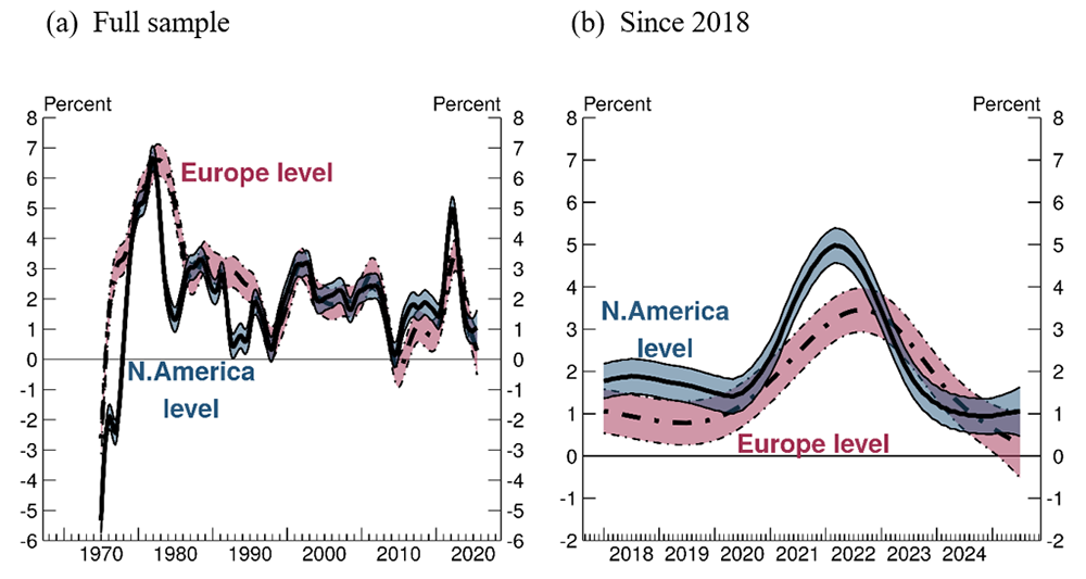
Note: Thick solid line and thick dot-dashed line show the estimated posterior means of the North America and Europe regional components, respectively. The thin solid and thin dot-dashed lines denote the edges of their respective 90% confidence intervals. Panel (A) plots the estimated Europe and North America regional components of core inflation over the from January 1975 to July 2025. Panel (B) plots these components since 2018.
Source: Authors' calculations.
More recently, as seen in Figure 1b, the North America regional component took off in 2021 and fell back the following year. Europe's regional component of core inflation also increased in 2021, but not as sharply as the North America component. And although the North America component was declining in 2022, the European component continued to rise that year.
The mean of the posterior distribution of the global component of core inflation is shown in Figure 2a. The global component of core inflation peaked in the 1970s and gradually declined through the 2000s. After the COVID pandemic, as shown in Figure 2b, the global component rose sharply, then partially retraced and has stabilized at around 1 3/4 percent, well above its average level of 1/4 percent in 2018-2019.
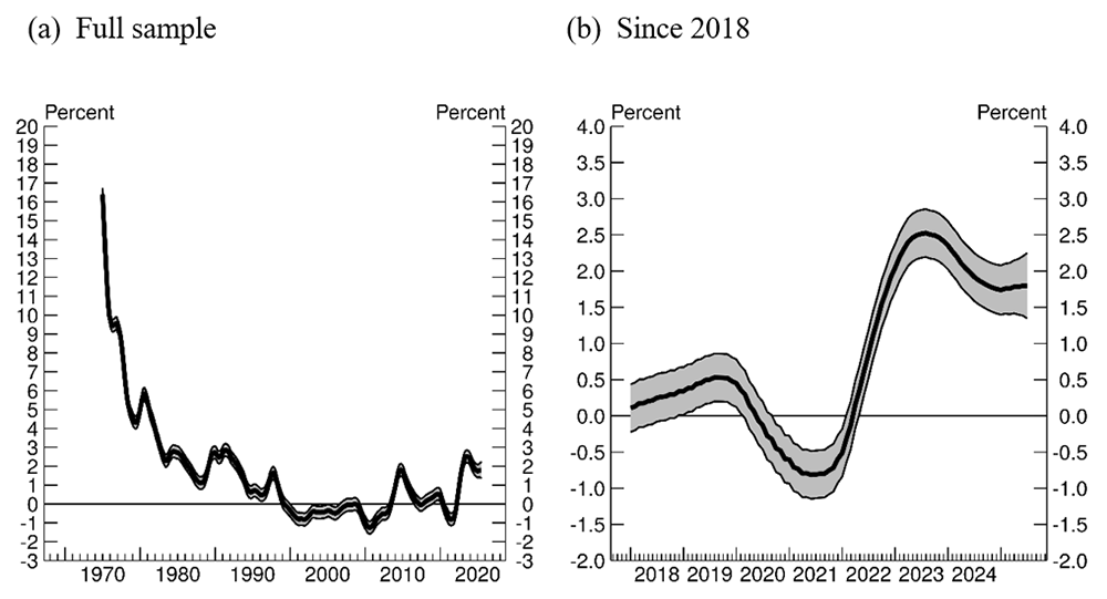
Note: Thick line shows the estimated posterior mean of the global component of core inflation. Thin lines denote the edges of its 90% confidence intervals. Panel (A) plots the estimated global component of core inflation from January 1975 to July 2025. Panel (B) plots this component since 2018.
Source: Authors' calculations.
Because our model allows the growth rates of the global and regional components to vary over time, we can assess the degree to which these components accelerated or decelerated following the COVID pandemic. As shown in Figure 3a, the global component's growth rate turns negative when the pandemic arrives in 2020, then shoots up as the global economy begins to reopen, before decelerating. The current growth rate has returned to zero, consistent with the flattening out of the global component at its still-elevated level. Figure 3b compares the growth rates of the regional components and shows a sharper acceleration and deceleration in core inflation in North America relative to Europe. While the North America growth rate has returned to zero, the growth rate in Europe remains negative, consistent with continued disinflation.
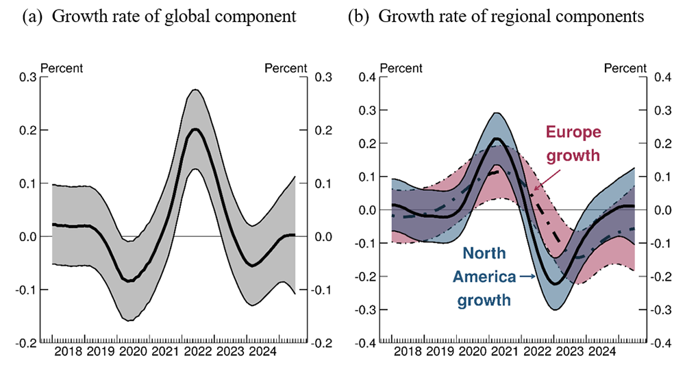
Note: Panel (A) plots the estimated growth rates of the global component, with the thick line denoting the posterior mean of the growth rate, and the thin line denoting the edges of the 90% confidence intervals. Panel (B) plots the estimated growth rates of the regional components. This solid line and thick dot-dash line show the estimated posterior means of the growth rates of the North America and Europe regional components, respectively. Thin solid and thin dot-dashed lines denote the edges of their respective 90% confidence intervals.
Source: Authors' calculations.
Using the estimated global, regional, and country-specific components, Figure 4 decomposes core inflation for the U.S., U.K., Canada, and France into the components described earlier. The country-specific components generally contribute less than the other components (with the exception of the U.K.) and are more volatile, as they capture the higher-frequency noise in core inflation for each country. The country-specific components also reflect differences in levels of core inflation between countries in the same region. For example, UK's core inflation was higher than that of the other European countries in our sample, resulting in a large positive estimated UK country-specific component. The opposite is true for France, which has had smaller rates of core inflation relative to the rest of Europe. In North America, the estimated country-specific component for the U.S. rises sharply in 2021, reflecting the sharper increase in U.S. core inflation relative to Canada's core inflation.
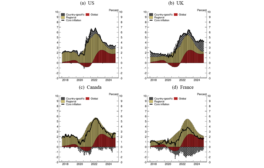
Note: Each panel decomposes core inflation for a given country. The solid black line is 12-month core inflation, also equal to the sum of the components. The bars represent the global, regional, and country-specific components.
Source: Authors' calculations.
3. Explaining the post-COVID surge in U.S. core inflation
Having extracted the regional, country-specific, and global components of core inflation for each country, we next examine their economic drivers, focusing on the global component and the North America regional component, which are the two largest components from the decomposition of U.S. core inflation shown in Figure 4a. We start by exploring the drivers of the global component, which is relatively large and shared by the other countries in our sample. To that end, we regress the 12-month change in the global component on a broad set of explanatory variables that proxy for global forces and then narrow the set of explanatory variables down to a parsimonious model using an automatic model selection tool.9 We underscore that this is our own research analysis based on our particular methodology and that different methodologies may produce different results.
The exercise yields a regression equation that fits the data well, with an adjusted R-squared of 0.77. Figure 5 shows the relative contributions of the drivers since 2019. The post-COVID surge in the global component is largely explained by global supply frictions as measured by changes in sea freight costs and global manufacturing backlogs (details in the figure), and to a lesser degree, past energy price shocks and overall tightness in labor markets across the countries in our sample.
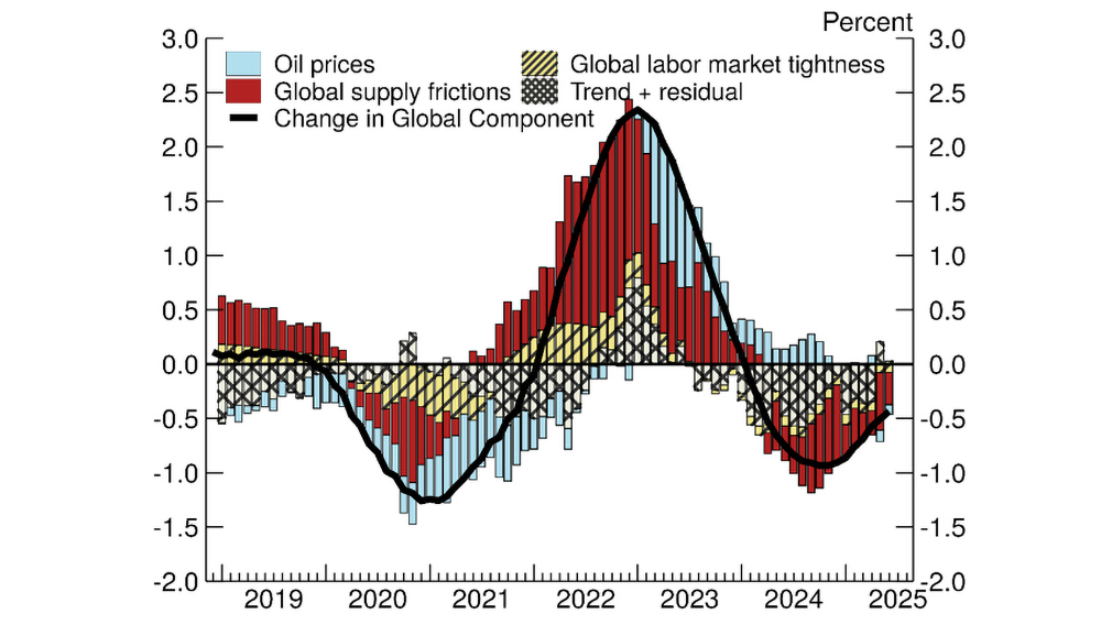
Note: This decomposition uses the estimated coefficients reported below,
$$ \Delta\mu_t^{Global}=-0.002t\ -0.278\ast\ Global \text{_} ugap_t+0.028\ast\Delta{SeaFreight}_t\ +0.033\ast\Delta{SeaFreight}_{t-12}$$
$$ +0.041 \ast Global \text{_} Manuf \text{_} Backlog_{t-6}+0.003\ast\Delta{Brent}_t^{Spot}\ +0.003\ast\Delta{Brent}_{t-24}^{Spot} $$
$$ +0.019\ast{Brent}_{t-12}^{Spot}+\ {\hat{\varepsilon}}_t, $$
and groups the contributions of the explanatory variables by broad category. Supply frictions include change in sea freight costs ($$SeaFreight$$) and global manufacturing backlogs ($$Global \text{_} Manuf \text{_} Backlog$$). The operator $$\Delta$$ denotes the twelve-month change. All coefficients are significant at the 5 percent level using heteroskedasticity and autocorrelation consistent standard errors.
Source: OECD Main Economic Indicators, S&P Global Purchasing Manager's Index (PMI), Current Population Survey, Producer Price Index, Organization of the Petroleum Exporting Countries, Japan Ministry of Health Labor and Welfare, Statistics Canada, Instituto Nazionale di Statistica, INSEE, Deutsche Bundesbank, UK Office for National Statistics, Statistics Austria, Instituto Nacional de Estatistica, Statistics Finland, Luxembourg Central Service of Statistics and Economic Studies, Statistics Netherlands; all via Haver Analytics.
We run a similar exercise to explain changes in the North America regional component, using data for the U.S. and Canada to construct regional averages of variables that measure labor market tightness and changes in consumption and savings.10 The results, shown in Figure 6, suggest that the surge in the North America regional component was largely driven by tightness in labor markets (regional changes in job-openings-to-unemployment ratio and average weekly earnings), and lagged changes in households' savings behavior (as excess savings during the pandemic boosted consumption spending).11
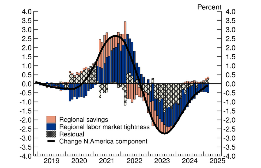
Note: This decomposition uses the estimated coefficients reported below
$$ \Delta\mu_t^{N.Amer.}=2.851\ast\Delta VU \text{_} ratio_t^{N.Amer.}+0.216\ast\ \Delta Weekly \text{_} earnings_t^{N.Amer.}+ $$
$$ 0.090\ast\Delta Pers \text{_} savings \text{_} rate_{t-12}^{N.Amer.}+\ {\hat{\varepsilon}}_t, $$
and groups the contributions of change in openings-to-unemployment ($$VU \text{_} ratio$$) and average weekly earnings ($$Weekly \text{_} earnings$$) into the labor market tightness category. Explanatory variables are the averages for the U.S. and Canada. The operator $$\Delta$$ denotes the twelve-month change. All coefficients, except the one on supplier delivery times, are significant at the 5 percent level using heteroskedasticity and autocorrelation consistent standard errors.
Source: OECD Main Economic Indicators, Current Employment Statistics, Current Population Survey, Job Openings and Labor Turnover Survey, National Income and Product Accounts; all via Haver Analytics.
4. Conclusion
We examine the international co-movement of core inflation from a regional perspective, using a Bayesian dynamic linear model that decomposes core inflation rates in the major advanced economies since the 1970s into global, regional, and country-specific components. We find that the post-pandemic surge in the global component largely reflected global supply frictions and to a lesser degree, past energy price shocks and overall tightness in labor markets across many countries. Meanwhile, the surge in the North America component is largely driven by tightness in labor markets and lagged changes in households' savings behavior.
Our results could have implications for monetary policy. Monetary policy could be challenging when the global and regional components of core inflation are moving in opposite directions. For example, in the second half of 2022, the regional component of U.S. core inflation had levelled off and started to decline, but this decline was masked by continued increases in the global component, leaving overall core inflation little changed at elevated levels.12
References
Aladangady, Aditya, David Cho, Laura Feiveson, and Eugenio Pinto, "Excess Savings during the COVID-19 Pandemic," FEDS Notes 2022-10-21, Board of Governors of the Federal Reserve System (U.S.) Oct 2022.
Alp, Harun, Matthew Klepacz, and Akhil Saxena, "Second-Round Effects of Oil Prices on Inflation in the Advanced Foreign Economies," FEDS Notes, Washington: Board of Governors of the Federal Reserve System 2023.
Cascaldi-Garcia, Danilo, Luca Guerrieri, Matteo Iacoviello, and Michele Modugno, "Lessons from the co-movement of inflation around the world," FEDS Notes, Washington: Board of Governors of the Federal Reserve System 2024.
Ciccarelli, Matteo and Benoˆıt Mojon, "Global inflation," Review of Economics and Statistics, 2010, 92 (3), 524–535.
Doornik, Jurgen A., "Encompassing and Automatic Model Selection," Oxford Bulletin of Economics and Statistics, December 2008, 70 (s1), 915–925.
_ , "Autometrics," in Jennifer Castle and Neil Shephard, eds., The Methodology and Practice of Econometrics: A Festschrift in Honour of David F. Hendry, Oxford University Press, 2009.
Foörster, Marcel and Peter Tillmann, "Reconsidering the International Comovement of Inflation," Open Economies Review, 2014, 25, 841–863.
Hendry, David F. and Jurgen A. Doornik, Empirical Econometric Modelling using PcGive: Volume I, London: Timberlake Consultants Press, 2009.
Mumtaz, Haroon, Saverio Simonello, and Paolo Surico, "International Comovements, Business Cycle and Inflation: a Historical Perspective," Review of Economic Dynamics, 2011, 14 (1), 176–198.
Negro, Marco Del, Domenico Giannone, Marc P. Giannoni, and Andrea Tam- balotti, "Global trends in interest rates," Journal of International Economics, 2019, 118, 248–262.
Parker, Miles, "How global is 'global inflation'?," Journal of Macroeconomics, 2018, 58, 174–197.
Petris, Giovanni, "An R Package for Dynamic Linear Models," Journal of Statistical Software, 2010, 36 (12), 1–16.
_, Sonia Petrone, and Patrizia Campagnoli, Dynamic Linear Models with R useR!, Springer-Verlag, New York, 2009.
Stock, James H. and Mark W. Watson, "Why Has U.S. Inflation Become Harder to Forecast?," Journal of Money, Credit and Banking, 2007, 39 (1), 3–33.
1. We thank Shaghil Ahmed, Danilo Cascaldi-Garcia, Thiago Ferreira, Luca Guerrieri, Matteo Iacoviello, participants of the GW forecasting seminar, and other colleagues at the Federal Reserve Board for comments and suggestions. Annika Johnson provided outstanding research assistance. The views expressed in this note are solely the responsibility of the authors and should not be interpreted as reflecting the views of the Board of Governors of the Federal Reserve System or of anyone else associated with the Federal Reserve System. Return to text
2. For a detailed description of the model and data see Beltran, Daniel and Julio Ortiz, 2025, "Core Inflation in the Advanced Economies; A Regional Perspective." International Finance Discussion Paper, forthcoming. Return to text
3. There is a large literature devoted to the international co-movement of inflation and the identification global inflation cycles. Ciccarelli and Mojon (2010) argue that inflation in OECD countries has been dominated by common shocks since the 1960s, and their measure of global inflation explain more than two-thirds of the variability in headline CPI inflation in these countries. Mumtaz et al. (2011) finds that regional factors account for the bulk of the fluctuations in both inflation and output growth in most countries. Using a richly specified dynamic hierarchical factor model, Förster and Tillmann (2014) find the opposite: global factors play only a minor role in explaining national inflation rates. Return to text
4. The 12 advanced economies are Germany, Italy, France, Portugal, Netherlands, Luxembourg, Finland, Austria, United Kingdom, United States, Canada, and Japan. Return to text
5. We use core consumer prices rather than headline consumer prices in part because the global component obtained from a decomposition of headline inflation would likely reflect energy and other commodity price fluctuations. By instead focusing on core inflation, which is often regarded as a strong signal for future headline inflation, our results could have more direct monetary policy implications. In particular, to the extent that energy and other commodity prices are important determinants of any of our estimated components, it is due to the passthrough of these prices to core consumer prices. Return to text
6. Stock and Watson (2007) model U.S. inflation dynamics as a univariate time series and find that U.S. CPI inflation is well described by an integrated moving average process of order 1, which is equivalent to an unobserved components model in which inflation has a stochastic trend that follows a random walk. We adopt a similar time-series specification but in a multivariate setting, and include both a stochastic global trend that is common to all the countries in the sample as well as a stochastic regional trend that is common to just the countries in the same region. Return to text
7. Our model assumes that regional innovations are orthogonal. We examined the sensitivity of our findings to this assumption by estimating a version of our model in which we allow the Europe and North America regional innovations to be correlated. We find that our results are qualitatively unchanged. Return to text
8. The model is written in state-space form and the posterior means of the global, regional, and country-specific components are estimated recursively using the Kalman filter (Petris et al., 2009). We ignore the estimated posterior means during the first 4 years of our sample to allow the Kalman filter to converge. The Bayesian approach with conjugate Normal priors facilitates the recursive estimation of the posterior means and variances of the global, regional, and country-specific components directly using the Kalman filter. To calibrate our priors for the state vector at time t=0, we use the global and regional averages of the 12-month core inflation rates from December 1970 (before the start of our estimation period), with wide confidence bands to make them less informative. Our results are robust to the choice of priors. The R package 'dlm' by Petris (2010) is used for estimation. The 19 deep parameters of the model—the variances of the regional and country-specific shocks, and the moving average coefficients for each country, and the autoregressive decay parameters for the growth shocks— are calibrated at their maximum likelihood estimates. Return to text
9. Specifically, we adopt a general-to-specific model selection strategy that begins with a 'general unrestricted model' (GUM) that encompasses the essential characteristics of the underlying data, and then eliminate variables that are statistically insignificant using Autometrics, which is part of the software package PcGive-OxMetrics (Doornik, 2009; Hendry and Doornik, 2009). Autometrics uses a tree-search algorithm to detect and eliminate statistically insignificant variables, avoiding path-dependence. At any stage, a variable is only removed if the new model encompasses the GUM. The terminal model is, by design, a statistically well-specified valid reduction of the GUM (Doornik, 2008). Return to text
10. We ran a similar regression to explain the 'non-global' part of U.S. core inflation by replacing the dependent variable with the sum of the 12-month change in the North America regional and U.S. country-specific components (using the same explanatory variables) and found similar results. Return to text
11. Aladangady et al. (2022) find that spending among U.S. households in the bottom half of the income distribution rises by about 10 percent above its pre-pandemic trend following the CARES Act in 2020 and remains well above trend through 2022. Return to text
12. In a speech at the time, Federal Reserve Chair Jerome Powell acknowledged that core inflation had "mainly moved sideways" and that "despite tighter policy and slower growth over the past year, we have not seen clear progress on slowing inflation. "Jerome H. Powell, 2022, "Inflation and the labor market'', Hutchins Center on Fiscal and Monetary Policy, Brookings Institution, Washington D.C., November 30. https://www.federalreserve.gov/newsevents/speech/powell20221130a.htm Return to text
Beltran, Daniel O., and Julio L. Ortiz (2025). "Inflation's Shared DNA: Regional and Global Factors in Post-Pandemic Core Inflation," FEDS Notes. Washington: Board of Governors of the Federal Reserve System, September 19, 2025, https://doi.org/10.17016/2380-7172.3888.
Disclaimer: FEDS Notes are articles in which Board staff offer their own views and present analysis on a range of topics in economics and finance. These articles are shorter and less technically oriented than FEDS Working Papers and IFDP papers.