FEDS Notes
March 31, 2022
Is Trend Inflation at Risk of Becoming Unanchored? The Role of Inflation Expectations
Danilo Cascaldi-Garcia, Francesca Loria, and David López-Salido1
Since the start of the pandemic, views about the evolution of aggregate consumer prices moved swiftly from concerns about deflation to fears about excessive inflation. It is hard to find a parallel in the history of the U.S. economy—or the global economy more generally—to this rapid reversal of risks to the inflation outlook. In this note, we estimate a monthly model of trend inflation in the United States and show that recent readings on inflation and inflation expectations suggest upward changes in its (long-run) trend.
We borrow the empirical framework presented in Mertens (2016), which we update using data up to March 2022. This empirical model is particularly well-suited to assess the extent to which longer-run inflation expectations are anchored and to detect episodes in which people's beliefs about the (longer-run) nominal anchor shift. This long-run anchor or trend reflects the public confidence in the central bank's commitment to price stability. In the model, the underlying inflation trend is captured by survey measures of inflation expectations, which may in turn be affected by beliefs about the conduct of monetary policy in the far future. To be more precise, we use this statistical model to estimate the inflation's long-run trend by taking signal from three inflation measures: past inflation, trimmed-mean inflation, and short- and long-term survey measures of inflation expectations or inflation forecasts.
The basic idea behind the identification of trend (core PCE) inflation is to construct a "stable" measure of inflation expectations over a period far enough in the future so that this measure is dominated by the central bank's commitment to achieving and maintaining a low and stable inflation rate rather than cyclical factors or other influences—such as relative price shocks, financial market participants' sentiments, or risk premiums. If this measure of trend (or underlying) inflation moves above the Federal Reserve's 2 percent longer-run goal, we may take it as an indication of a "level de-anchoring" in long-term inflation expectations.
The empirical model allows to quantify another interesting aspect of underlying inflation, namely the "uncertainty" associated with the estimates of trend inflation. This uncertainty measure provides a criterion for evaluating the extent to which long-run (trend) inflation remains well anchored: whenever the uncertainty regarding estimated trend inflation is large, it indicates a "risk of de-anchoring" of longer-run inflation expectations.
The model can thus give insights into whether movements in inflation determinants result in a level and/or risk-uncertainty shift in longer-run inflation and longer-run inflation expectations.
1. Model specification and data
In the model, trend inflation $$\tau_t$$ is defined as the infinite-horizon forecast of inflation $$(\pi_t)$$ conditional on a given information set $$\Omega_t$$ (e.g., past inflation, trimmed-mean inflation, and survey measures of inflation expectations).2 Formally, $$\tau_t=E\left(\pi_{t+\infty}\right|\Omega_t)$$. Insofar as the trend inflation rate amounts to the forecast of what inflation will be at a fixed point, very far in the future, changes in trend inflation merely reflect changes in information—not changes in the horizon.
This definition of trend inflation implies that it follows a unit root process, since
$$$$E\left(\pi_{t+\infty}\right|\Omega_t)-\ E\left(\pi_{t+\infty}\right|\Omega_{t-1})=\tau_t-\ \tau_{t-1}$$$$
and thus
$$$$\tau_t=\ \tau_{t-1}+\ E\left(\pi_{t+\infty}\right|\Omega_t)-\ E\left(\pi_{t+\infty}\right|\Omega_{t-1})=\ \tau_{t-1}+\ \bar{e_t}$$$$
where $$\bar{e_t} \sim N(0,\ {\bar{\sigma}}_t^2)$$ is a sequence of shocks to trend with time-varying volatility $${\bar{\sigma}}_t^2$$. Actual inflation is modeled as the sum of this trend and a stationary component $$\widetilde{\pi_t}$$ and inherits the random walk in the trend: $$\pi_t=\ \tau_t+\ \widetilde{\pi_t}$$.3
The shocks to the trend, $$\bar{e_t}$$, have an important economic interpretation. When there are no shocks, trend inflation remains stable, it is equal to its past value, and under these circumstances the longer-run "level" of inflation expectations is well-anchored. However, when these "trend (or permanent) shocks" are sizable, the current inflation trend drifts away from its previous level, implying a potential shift in inflation expectations. When the uncertainty associated with these trend shocks is large, there is an indication of inflation expectations becoming de-anchored. The greater is this uncertainty, the larger is the "risk of de-anchoring."
In this framework, the inflation trend is an unobserved component of current inflation. However, what the econometrician observes is a set of indicators that might be informative about such trend or underlying component of inflation.4 In what follows, we focus on an empirical model that takes signal from the following indicators:
- Past inflation: Actual inflation rates, changes in CPI and PCE indexes, and the GDP deflator.
- Trimmed-mean inflation: Median and trimmed measures of CPI and PCE realized inflation.
- Surveys: Forecasts of future inflation obtained from the Survey of Professional Forecasters (SPF), the Blue Chip, and the Livingston Survey.
Table A.1 of the Appendix summarizes the specific inflation measures of each category that inform the estimation of core PCE trend inflation in our model.
2. Results
This section discusses the key results arising from the estimation of core PCE trend inflation, $$\tau_t$$, and its time-varying uncertainty $$\bar{\sigma_t}$$. The level of the trend is measured in annualized percentage points and uncertainty is measured by the standard deviation of the trend shock $$\bar{e_t}$$.
The estimates of the baseline version of our model uses data from January 2000 up to March 2022,5 with data on past inflation, trimmed inflation, and survey measures of inflation. The baseline model includes data on past inflation, trimmed inflation and survey measures of inflation. As we show later in this note, the estimation of this baseline model using data from the most recent decades produces the best forecasting performance—compared with competing alternative models that only use a subset of inflation measures (i.e., "past inflation only," "trimmed-mean only," and "surveys only").6
Figure 1 shows the evolution of the estimated trend inflation $$\tau_t$$, on the left panel, and its uncertainty $$\bar{\sigma_t}$$ on the right panel, since January 2008. Thick lines denote posterior means and thin lines depict 90 percent credible sets around the posterior means. Shaded areas indicate NBER-dated recessions. Core PCE trend inflation witnessed a notable decline below its post-2000 average during the COVID-19 recession, but it is showing a substantial rebound during the recovery—with the current estimate of the trend above 2 percent.
The uncertainty $$\bar{\sigma_t}$$ associated with the trend $$\tau_t$$ has steadily declined after its peak in 2012, but the recovery from the COVID-19 recession moved it up to levels above its historical average. Taken altogether, these results suggest upward risks to trend inflation in terms of both its level and its variance.
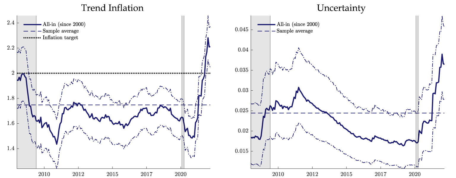
Note: Panel on the left depicts the estimated trend core PCE inflation (blue solid line), taking signal from past inflation, trimmed-mean inflation, and survey forecasts, with sample from Jan/2000 to Mar/2022. Dotted line represents the 2 percent inflation target. Panel on the right depicts the estimated uncertainty of the trend inflation. Dashed blue lines in each panel represent the sample average of the trend inflation and of the uncertainty, respectively. Dot-dashed blue lines represent a 90% coverage band of the trend inflation and of the uncertainty, respectively. Shaded gray bars indicate periods of business recession as defined by the National Bureau of Economic Research (NBER): December 2007 to June 2009, and February 2020 to April 2020.
3. A counterfactual exercise
Next, we use our baseline model to study how trend inflation would change in a counterfactual "stress" scenario where inflation expectations deteriorate considerably. More specifically, this exercise envisions a situation in which inflation expectations increase substantially over the remainder of the year and stay high up to September 2022. The size of this increase in inflation expectations corresponds to a shock of two standard deviations of the distribution of inflation calculated over the past 20 years. Table 1 describes the details of how this scenario is implemented.
Table 1: Counterfactual Assumptions
| Variable | Scenario |
|---|---|
| Inflation measures | |
| PCE inflation (trimmed) | 3.5% y.o.y. (Sep/2022) |
| CPI Inflation (trimmed) | 6.5% y.o.y. (Sep/2022) |
| CPI Inflation (median) | 6.3% y.o.y. (Sep/2022) |
| Surveys | |
| SPF short-run – PCE core inflation (two years ahead) | 2.50% |
| SPF short-run – CPI core inflation (two years ahead) | 2.70% |
| SPF short-run – PCE inflation (up to four quarters ahead) | 2.6%-4.0% |
| SPF short-run – CPI inflation (up to four quarters ahead) | 2.9%-4.8% |
| SPF short-run – GDP deflator (up to four quarters ahead) | 6.6%-7.5% |
| SPF long-run – PCE inflation (5 to 10 years) | 2.4%-2.7% |
| SPF long-run – CPI inflation (5 to 10 years) | 2.7%-3.1% |
| Blue Chip –CPI inflation (short and long-run) | 2.5%-2.9% |
| Blue Chip – GDP deflator (short and long-run) | 2.2%-3.1% |
| Livingston Survey – CPI inflation (12 months ahead) | 3.30% |
Extending the sample period with these counterfactual "data" in hand, we use the empirical model to estimate the corresponding level and uncertainty of trend inflation over the next few quarters. Figure 2 displays the results, focusing on the period starting in January 2016. The figure reveals that, under the configuration of inflation data and survey measures considered in this thought experiment, the model would indicate a prolonged increase in trend inflation (left panel) to about 2.5 percent (annualized) and sustained high trend-inflation uncertainty (right panel). Such a scenario suggests a significant increase in the risk of a de-anchoring of trend inflation to heights well above its historical average over the last 20 years. This exercise highlights the kind of magnitude and persistence of a shock to survey measures of inflation expectations that would reflect trend inflation significantly above the 2 percent inflation target and would prompt substantial risk to de-anchoring long-run inflation.
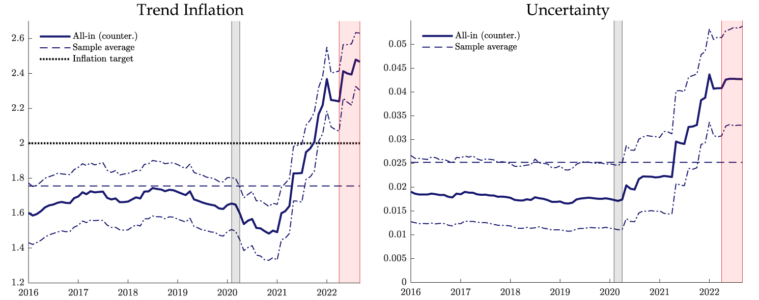
Note: Panel on the left depicts the estimated trend core PCE inflation (blue solid line), taking signal from past inflation, trimmed-mean inflation, and survey forecasts, with counterfactual sample from Jan/2000 to Sep/2022. Dotted line represents the 2 percent inflation target. Panel on the right depicts the estimated uncertainty of the trend inflation. Dashed blue lines in each panel represent the sample average of the trend inflation and of the uncertainty, respectively. Dot-dashed blue lines represent a 90% coverage band of the trend inflation and of the uncertainty, respectively. Shaded gray bars indicate periods of business recession as defined by the National Bureau of Economic Research (NBER): February 2020 to April 2020. Shaded red bars represents the counterfactual period (Apr/2022 to Sep/2022).
Importance (over time) of survey measures of expectations
We now explore the relative forecasting ability of our baseline model considered above, as well as competing models. Specifically, we focus on the following four models:
- Past Inflation Model: Only includes realized inflation rates, like those derived from the CPI, PCE, and GDP deflator.
- Trimmed Model: Only includes trimmed-mean or median measures of realized inflation.
- Surveys Model: Only includes survey forecasts of future inflation obtained from the Survey of Professional Forecasters (SPF), the Blue Chip, and the Livingston surveys.7
- "All-in" (Baseline) Model: Includes a combination of realized inflation rates, trimmed-mean and median measures, and survey forecasts.
We also consider results for three different sample periods: (i) full sample (Jan/1960 – Mar/2022), (ii) pre-2000s (Jan/1960 – Dec/1999), and iii) recent periods (Jan/2000 – Mar/2022). The 2000 cutoff has been chosen as both the level and the variability of trend inflation are lower since then compared to previous years.
Table 2 reports root-mean-squared errors (RMSEs) for the "naïve" past-inflation trend model. For all other models, it shows the ratio of their RMSEs relative to those of the "naïve" past-inflation trend model. RMSEs are computed as the difference between forecasts and realized values of average PCE core inflation over different horizons. The lower the RMSE of a model, the better its forecasting performance. As to the RMSE ratios, a number below 1 means that the forecasting performance of a given alternative measure is better than that of the "naïve" model (which draws on the behavior of past inflation and no other series).
Three results stand out. First, in the most recent subsample, after 2000, characterized by low inflation volatility, the forecasting ability of all models improves upon models estimated over the full sample, or the first subsample (1960-1999). Second, although in the pre-2000s subsample the results favor the "trimmed-mean and median measures" model, in the recent subsample, after 2000, the use of survey measures of inflation clearly proves extremely useful in forecasting trend inflation. Finally, our baseline model estimated over the most recent sample of data performs best.
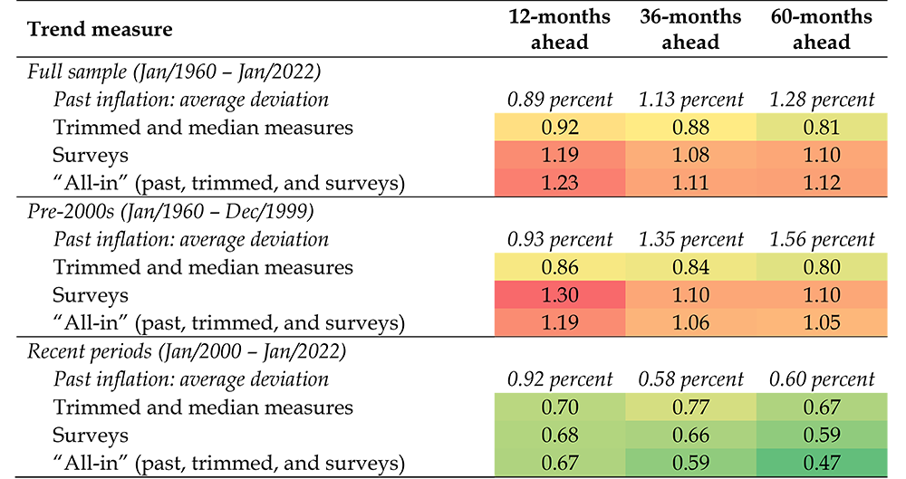
Note: Root-mean-squared errors (RMSEs) are in levels for the "naïve" past-inflation trend model. For all other models, the table reports the ratio of their RMSEs relative to those of the "naïve" past-inflation trend model. RMSEs are computed as the difference between forecasts and realized values of average PCE core inflation over different horizons. RMSE evaluation restricted to Jan/2022 due to PCE inflation availability.
References
Blanchard, O., Cerutti, E., & Summers, L. (2015). Inflation and Activity – Two Explorations and Their Monetary Policy Implications (No. w21726). National Bureau of Economic Research.
López-Salido, J. D., & Loria, F. (2020). Inflation at Risk. Finance and Economics Discussion Series 2020-013, Board of Governors of the Federal Reserve System (U.S.).
Mertens, E. (2016). Measuring the Level and Uncertainty of Trend Inflation. Review of Economics and Statistics, 98(5), 950-967.
McLeay, M., & Tenreyro, S. (2020). Optimal Inflation and the Identification of the Phillips Curve. NBER Macroeconomics Annual, 34(1), 199-255.
Appendix
Table A.1 summarizes the data used in our analysis. Figures A.1 and A.2 show the time series estimates of trend inflation and uncertainty of the stochastic trend obtained using the full sample, 1960-2022, for the “past inflation,” “trimmed,” “surveys,” and “all-in (baseline)” models.
Table A.1: Data Description and Availability
| Since | Until | Frequency | ||
|---|---|---|---|---|
| Realized Inflation Rates | ||||
| PCE deflator | Feb-59 | Jan-22 | Every month | |
| Core PCE deflator (ex. food and energy) | Feb-59 | Jan-22 | Every month | |
| Consumer price index | Feb-47 | Feb-22 | Every month | |
| GDP deflator | Q1/1947 | Q3/2021 | Mar, Jun, Sep, Dec | |
| Trimmed and Median Inflation Rates | ||||
| Trimmed-mean PCE inflation | Jan-78 | Jan-22 | Every month | |
| Trimmed-mean and Median CPI inflation | Jan-83 | Feb-22 | Every month | |
| Survey Expectations of Inflation | ||||
| SPF short-term forecasts | Core PCE and Core CPI, next two years | Feb-07 | Feb-22 | Feb, May, Aug, Nov |
| PCE and CPI, avg. over the next four quarters | Feb-07 | Feb-22 | Feb, May, Aug, Nov | |
| GDP/GNP deflator, avg. over the next year | Nov-68 | Feb-22 | Feb, May, Aug, Nov | |
| SPF longer-term forecasts | PCE, next five and next ten years | Feb-07 | Feb-22 | Feb, May, Aug, Nov |
| CPI, next five years | Aug-05 | Feb-22 | Feb, May, Aug, Nov | |
| CPI, next ten years | Nov-79 | Feb-22 | Feb, May, Aug, Nov | |
| Blue Chip, five-to-ten years ahead | CPI and GDP/GNP deflator | Mar-86 | Oct-21 | Mar, Oct |
| Blue Chip, four quarters ahead | CPI | Jun-80 | Mar-22 | Every month |
| GDP/GNP deflator | Jun-80 | Mar-22 | Every month | |
| Livingston, 6–12 months ahead | Jun-60 | Dec-21 | Jun, Dec | |
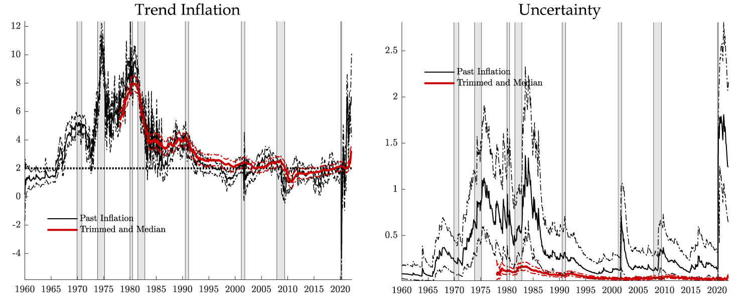
Note: Left panel depicts the estimated trend core PCE inflation, with solid black line representing a model that takes signal only from past inflation, and solid red line representing a model that takes signal only from trimmed-mean inflation, both with sample from Jan/1960 to Mar/2022. Dotted line represents the 2 percent inflation target. Panel on the right depicts the estimated uncertainty of these two trend inflations. Dot-dashed black and dot-dashed red lines represent a 90% coverage band of the trend inflation and of the uncertainty, respectively. Shaded gray bars indicate periods of business recession as defined by the National Bureau of Economic Research (NBER): December 1969 to November 1970, November 1973 to March 1975, January 1980 to July 1980, July 1981 to November 1982, July 1990 to March 1991, March 2001 to November 2001, December 2007 to June 2009, and February 2020 to April 2020.
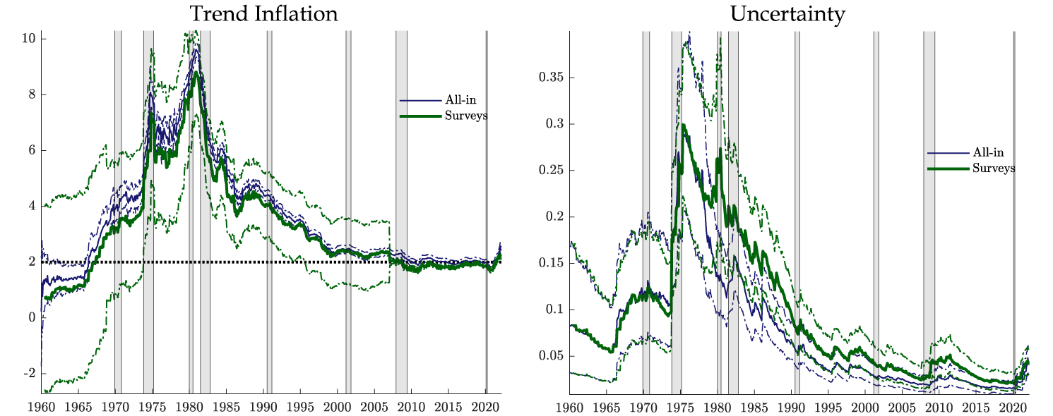
Note: Left panel depicts the estimated trend core PCE inflation, with solid blue line representing a model that takes signal from past inflation, trimmed-mean inflation, and survey forecasts, and solid green line representing a model that takes signal only from surveys, both with sample from Jan/1960 to Mar/2022. Dotted line represents the 2 percent inflation target. Panel on the right depicts the estimated uncertainty of these two trend inflations. Dot-dashed blue and dot-dashed green lines represent a 90% coverage band of the trend inflation and of the uncertainty, respectively. Shaded gray bars indicate periods of business recession as defined by the National Bureau of Economic Research (NBER): December 1969 to November 1970, November 1973 to March 1975, January 1980 to July 1980, July 1981 to November 1982, July 1990 to March 1991, March 2001 to November 2001, December 2007 to June 2009, and February 2020 to April 2020.
1. We thank Jim Clouse, Andrea de Michelis, Andrea Raffo, Ed Nelson, Trevor Reeve, Stacey Tevlin, and Beth Anne Wilson for comments on an earlier draft. The views expressed in this note are solely the responsibility of the authors and should not be interpreted as reflecting the views of the Board of Governors of the Federal Reserve System or of anyone else associated with the Federal Reserve System. Replication code is available from the authors upon request. Return to text
2. Trend inflation intends to capture long-run inflation, or the rate that would prevail in the absence of resource slack, supply shocks, and other temporary disturbances to inflation. While similar in spirit, common inflation focuses on short-run movements, determining how much of a current change in prices is driven by macroeconomic factors, as opposed to idiosyncratic developments or measurement error. Return to text
3. In the model, whether actual inflation is described by a stationary or nonstationary process is ultimately a result of how much weight it assigns to the nonstationary component coming from the trend and to the stationary component (i.e., the size of the time-varying volatility $$\ {\bar{\sigma}}_t^2)$$ . Return to text
4. The model is a generalization of the univariate Stock and Watson (2005) unobserved components model with stochastic volatility. The model takes signal from a large set of observables and allows for missing observations arising from the use of mixed frequency in the data. Return to text
5. PCE inflation is only available up to January 2022, see Table A.1 in the Appendix. Return to text
6. Figures A.1 and A.2 in the Appendix present the full sample (since January 1960) time series for the trend and volatility for all models. Return to text
7. See Blanchard, Cerutti, and Summers (2015), McLeay and Tenreyro (2020), and López-Salido and Loria (2020). Return to text
Cascaldi-Garcia, Danilo, Francesca Loria, and David López-Salido (2022). "Is Trend Inflation at Risk of Becoming Unanchored? The Role of Inflation Expectations," FEDS Notes. Washington: Board of Governors of the Federal Reserve System, March 31, 2022, https://doi.org/10.17016/2380-7172.3043.
Disclaimer: FEDS Notes are articles in which Board staff offer their own views and present analysis on a range of topics in economics and finance. These articles are shorter and less technically oriented than FEDS Working Papers and IFDP papers.