Board of Governors of the Federal Reserve System

October 19, 2018

Optimal Monetary Policy in a DSGE Model with Attenuated Forward Guidance Effects

Hess Chung, Taisuke Nakata, and Matthias Paustian¹

1. Introduction
When current policy rates are at the effective lower bound (ELB), central banks often turn to communication about the future path of policy rates--known as forward guidance--as an alternative means to influence economic activity. According to standard sticky-price dynamic stochastic general equilibrium (DSGE) models often used in academia and by central banks to analyze monetary policy, forward guidance is a powerful substitute for a change in the current policy rate and should be used by central banks to improve welfare when the current policy rate is constrained by the ELB.² In particular, in these models, the central bank finds it optimal to announce that it will keep the policy rate at the ELB for longer than would be warranted when considering future output and inflation stabilization alone.

A number of papers have recently pointed out an intriguing feature of this standard model: The economic effects of forward guidance can be implausibly large.³ This feature--often referred to as the forward guidance puzzle--has generated concern among researchers that the standard model is of limited use for the analysis of forward guidance policies and, as a result, has generated an interest in modifying the standard model to attenuate the implausibly large effects of forward guidance.

In this article, we explore the implications of attenuating the power of forward guidance for the optimal conduct of forward guidance policy in a quantitative DSGE model of the U.S. economy. The main takeaway of our analysis is that when forward guidance is less powerful, it is typically optimal for the central bank to compensate for the reduced power of forward guidance by using it more aggressively.

2. What is the Forward Guidance Puzzle?
Standard economic theory prescribes that households and firms should take future economic conditions into account when making their decisions today. In particular, the household consumption–saving decision should be sensitive to the expected path of real interest rates, which define the opportunity cost of current consumption relative to consumption in future periods. Similarly, under the common assumption that resetting prices is costly, firms should take into account future demand conditions when setting their prices now.

In the context of the New Keynesian models typically used at central banks, these forward-looking features have surprising implications for the effects of anticipated monetary policy actions. We demonstrate these features by starting with the observation that, absent any financial market frictions, an optimizing household should choose its consumption path to equate the value of additional consumption today with the value (perceived today) of deferring that additional consumption to some later time. This principle is formalized in the Euler equation

$$$$ \lambda_t = \beta^{T-t} (r_{t+1} r_{t+2}\dots r_T ) \lambda_T ,$$$$

where $$\lambda_t$$ is the marginal utility of consumption at time t, $$\beta$$ represents the household's rate of time preference, and $$r_t$$ is the real rate of return between time t-1 and t.⁴ In the long run, temporary demand shocks, such as monetary policy interventions, cannot have real effects on aggregate variables and so, if we take T large enough, $$\lambda_T$$ should be approximately independent of any such shocks that occur for times much earlier than T. Therefore, a 1 percentage point decrease in the real interest rate at any single time in the future, no matter how far in advance, should lead to the same 1 percent decrease in the marginal utility of consumption and because this marginal utility is closely tied to consumption itself, to similar rises in consumption.

This property of the Euler equation appears in conflict with intuition from permanent income theories of consumption where, conditional on income and current wealth, distant shocks to real interest rates should have smaller effects on current consumption than more proximal shocks. Indeed, as emphasized by Farhi and Werning (2017) and Angeletos and Lian (2018), the consumption function associated with the Euler equation for an individual household does have the property that consumption is less sensitive to distant interest rates, but this effect is offset by general equilibrium effects. In the canonical three-equation New Keynesian model, the farther into the future the interest rate movement occurs, the larger is the effect on permanent income and ultimately the discounting of future interest rates is exactly offset.

Moreover, in many DSGE models featuring costly price adjustment, the dynamics of inflation are represented by a New Keynesian Phillips curve of the form

$$$$ \pi_t = \kappa{MC}_t+\gamma\pi_{t+1}, $$$$

where $$\pi_t$$ is the inflation rate and $$MC_t$$ is the marginal cost.⁵ As is apparent from the Euler equation, an expected reduction in the monetary policy rate in the future stimulates aggregate demand in that and all prior periods, raising marginal costs and hence inflation at all prior times since price setters are forward looking. Higher inflation along the entire path (before the actual reduction in the policy rate) lowers real interest rates even further, which stimulates consumption along the entire path as indicated by the Euler equation. This process is explosive backwards in time: the farther in future the shock occurs, the stronger the effect on interest rates today. This feature of standard DSGE models--that an anticipated monetary policy shock far into the future has an implausibly large effect on today's economy--is often referred to as the forward guidance puzzle (Del Negro, Giannoni, and Patterson (2015) and Calstrom, Fuerst, and Paustian (2015)).

Figure 1: Impulse responses to unanticipated and expected monetary policy shocks under various assumptions about discounting

Y-axis: Fed Funds Rate and 4Q Inflation Rate are percentage points; Output is percent deviation.

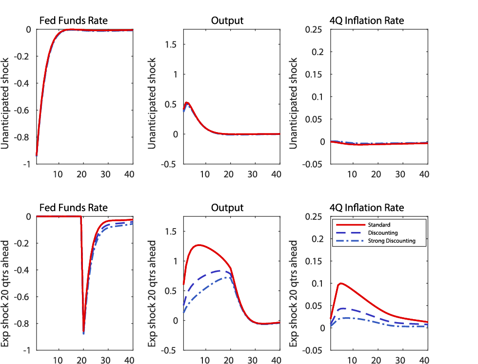
To illustrate this point, we use a version of the DSGE model developed by Del Negro, Giannoni, and Schorfheide (2015). We compare the effect of an unanticipated monetary policy rule shock on inflation and the level of output--shown by the red lines in the top row of Figure 1--with the effect of a monetary policy rule shock anticipated to occur 20 quarters into the simulation--shown by the red lines in the bottom row of Figure 1. To emphasize the mechanisms described earlier, we assume that the nominal interest rate prior to the shock is held fixed, as would naturally occur if the policy rate were constrained by its lower bound.⁶ While the unanticipated shock raises the level of output by around 1/2 percentage point, the anticipated shock raises the level of output by roughly 1 percentage point for almost the entire time prior to the shock's arrival. Similarly, while the unanticipated shock hardly moves inflation at all, the anticipated shock causes inflation to rise about 10 basis points above baseline several years before the shock is realized.

3. Attenuating the Forward Guidance Puzzle
The forward guidance puzzle present in standard DSGE models raises concerns about whether such models are a good framework for analyzing forward guidance policies, which are intended to influence today's economic activities by affecting the anticipated path of future federal funds rates. An active area of research in macroeconomics is to find sensible deviations from the standard DSGE framework that can reduce the power of forward guidance to a more plausible level. Over the last few years, researchers have produced a myriad of ways to reduce the power of forward guidance in DSGE models.⁷

As shown in this literature, a number of these attenuating factors can be approximated by the modifications to the Euler equation and the Phillips curve that we discussed earlier, as these two equations are at the heart of the forward guidance puzzle. For example, McKay, Nakamura, and Steinsson (2017) argue that the response to interest rate shocks in a model with idiosyncratic income shocks and constraints on borrowing can be closely matched by a "discounted Euler equation" of the form

$$$$ log(\lambda_t) = constant+(1-\alpha) log(\lambda_{t+1} )+log(r_{t+1} ), $$$$

where $$\alpha$$ is between 0 and 1. Iterating this equation forward, we obtain

$$$$ log(\lambda_t) = c+log(r_{t+1} )+(1-\alpha)log(r_{t+2} )+(1-\alpha)^2 log(r_{t+3} ) + \dots $$$$

The Euler equation shown earlier can be recovered if $$\alpha=0$$. When $$\alpha>0$$, as proposed by McKay, Nakamura, and Steinsson (2017), among others, the effect of shocks to expected real interest rates will have less and less effect on current consumption as the realization of those shocks is postponed further into the future. Similarly, in the Phillips curve, reducing the coefficient on expected inflation $$(\gamma)$$ below the household's rate of time preference can also limit or eliminate the amplification of demand shocks occurring far into the future.

To illustrate how discounting these expectations reduces the effects of future monetary policy shocks, the blue lines in Figure 1 show the effects of anticipated and unanticipated shocks in a model with a discounted Euler equation $$(\alpha=0.025)$$ and a (over)discounted Phillips curve $$(\gamma = \beta[1-0.0025])$$. Because a one-time shock to the policy rule has relatively transient effects in the standard model, the modest degree of discounting that we introduce makes little difference to the impulse response following an unanticipated shock. However, the effect of anticipated shocks on output and inflation is significantly attenuated.⁸ Clearly, the quantitative implications of discounting are sensitive to seemingly small variations in the parameters (see the difference between 0.025 and 0.05).

4. Implications of Attenuating the Power of Forward Guidance

We now turn to the main exercise of this article, which is to investigate the optimal policy implication of attenuating the forward guidance puzzle. We construct a recession scenario assuming that the federal funds rate is determined by a Taylor-type interest rate rule. Then, we examine how the recession looks if the central bank optimally chooses the federal funds rate path under commitment.⁹ We consider two economies with alternative degrees of discounting: one with a moderate degree of discounting $$(\alpha=0.025)$$ and the other one with a stronger degree of discounting $$(\alpha=0.05)$$.¹⁰ These two economies are contrasted with the standard model without any discounting $$(\alpha=0)$$. We conduct this experiment twice: first in the model that allows for discounting only in the Euler equation and second in the model that allows for discounting in both the Euler equation and the Phillips curve.

Figure 2 shows the results from the first experiment. The black lines show the evolution of the federal funds rate, the output gap, and inflation under the baseline rule (recall that, by construction, the recession scenario is identical across the three economies). Under the baseline rule, the output gap declines to minus 10 percent two years into the recession. Inflation declines by more than 1/2 percentage point. The federal funds rate stays at the ELB for 19 quarters.

The red, dark blue, and light blue lines show the optimal policy outcomes for the model without discounting, the model with moderate discounting, and the model with strong discounting, respectively. Regardless of the degree of discounting, under the optimal policy, the central bank keeps the federal funds rate at the ELB for longer than it does under the baseline rule. With the discounting parameter of 0, 0.025 and 0.05, the federal funds rate is kept at the ELB for 25 quarters, 27 quarters, and 30 quarters, respectively. This lower-for-longer policy rate path generates an overshooting of inflation throughout the simulation horizon and a temporary overshooting of the unemployment rate as the economy recovers. Since households and firms are forward looking, the expectations of the strong economy down the road help mitigate the decline in the output gap during the recession.

As shown by the red line, the power of forward guidance is implausibly strong in the model without discounting. Compared to the baseline rule, delaying the liftoff by a little more than a year can turn an extraordinarily severe recession with a 10 percent decline in output at the trough into a comparably mild downturn. Output barely falls on impact and even at the trough is only 2 percent below baseline. While the effects of the forward guidance policy in the aftermath of the financial crisis are uncertain, most observers would judge that the effect of interest rate policy depicted in this model is too strong.

Figure 2: A recession scenario and optimal outcomes under different assumptions about the discounting in the Euler equation

Y-axis: Percent

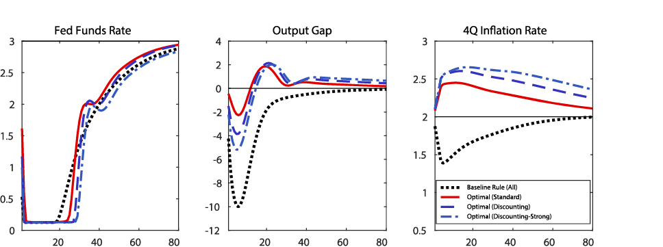
It is optimal for the central bank to keep the federal funds rate at the ELB for longer in the model with discounting than in the model without discounting. With the federal funds rate kept at the ELB for longer, the magnitude of the output overshooting is somewhat larger and the inflation overshooting is appreciably more severe. Note that, even though the federal funds rate stays at the ELB for longer in the model with discounting, the output gap declines by more. With the discounting of 0.025 and 0.05, the output gap declines to minus 4 percent and minus 5 percent at trough, respectively, as opposed to minus 2 percent in the standard model without discounting. Because households discount future income by more, the stronger real activity in the future is not as stimulative as in the model without discounting.

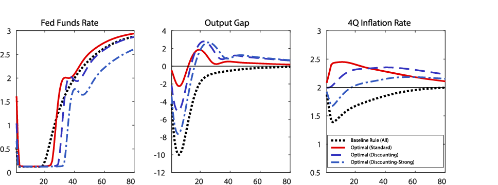
Figure 3 shows the results from the second experiment in which we introduce discounting to both the Euler equation and the Phillips curve. Consistent with what we saw in the first experiment, the central bank finds it optimal to keep the federal funds rate at the ELB for longer when the degree of discounting is larger. With the discounting parameter of 0.025 and 0.05, the ELB duration is 29 quarters and 33 quarters, respectively (versus 25 quarters in the model without discounting). Similarly to the first experiment, despite the longer ELB duration, the output gap declines by more in the model with discounting because households are less forward looking. With the discounting parameter of 0.025 and 0.05, the trough output gap is minus 5 percent and minus 7.5 percent, respectively. With price setters also discounting future inflation by more in this experiment, the optimal policy permits less inflation overshooting later and, as a result, inflation during the recession is lower than shown in Figure 2. Inflation declines by more than 30 basis points in the model with the discounting parameter of 0.05.

Figure 3: A recession scenario and optimal outcomes under different assumptions about the discounting in both the Euler equation and the Phillips curve

Y-axis: Percent

Why is it optimal for the central bank to keep the federal funds rate at the ELB for longer in the model with discounting? This result is an outcome of two competing forces. On the one hand, when the effects of future monetary policy adjustment on current economic conditions are smaller, the forward guidance policy has a smaller benefit for near-term outcomes while having similar costs in the future where it causes an overshoot of inflation and the output gap. That is, the central bank has an incentive to use forward guidance less aggressively. In our experiments, this logic means that the federal funds rate is kept at the ELB for a shorter period. On the other hand, when a future rate adjustment is less effective and the same reduction in a future policy rate leads to a smaller increase in today's inflation and output gap, it gives the central bank an incentive to promise to provide more accommodation in future because the central bank would not be able to meaningfully increase today's inflation and output gap otherwise. Which of these two competing incentives dominates depends on the specifics of the model. In the two experiments we show (and many other unreported experiments), the second incentive dominates the first. That is, the central bank finds it optimal to compensate for the reduced power of forward guidance by using it more aggressively.¹¹

5. Concluding Remarks
In this article, we have examined the implications of reducing the power of forward guidance for the optimal conduct of forward guidance policy. The key result is that it is optimal for the central bank to promise to keep the federal funds rate at the ELB for longer when forward guidance is less powerful.

As with any model-based analysis, caution is needed to interpret the policy implications of our analysis. In particular, an important caveat to our analysis is that it is semi-structural: We are silent about the model's primitives that justify the discounting in the Euler equation and the Phillips curve, and, as a result, our analysis is not immune to the Lucas critique (Cochrane (2016)). However, because many different micro-founded models of less powerful forward guidance end up with something that looks like the discounted Euler equation and Phillips curve, the insights from our analysis can be seen as providing a useful starting point for understanding optimal policy in those micro-founded models. We leave such structural analysis to future research.¹²

References
Angeletos, George-Marios, and Chen Lian (2018). "Forward Guidance without Common Knowledge," American Economic Review, vol. 108 (9), pp. 2477-512.

Carlstrom, Charles T., Timothy S. Fuerst, and Matthias Paustian (2015). "Inflation and Output in New Keynesian Models with a Transient Interest Rate Peg," Journal of Monetary Economics, vol. 76, pp. 230-43.

Chung, Hess (2015). "The Effects of Forward Guidance in Three Macro Models," FEDS Notes. Washington: Board of Governors of the Federal Reserve System, February 26, https://www.federalreserve.gov/econresdata/notes/feds-notes/2015/effects-of-forward-guidance-in-three-macro-models-20150226.html.

Cochrane, John (2016). "Comments on 'A Behavioral New Keynesian Model,'" unpublished paper. Hoover Institution. https://faculty.chicagobooth.edu/john.cochrane/research/papers/gabaix_comments.pdf

Del Negro, Marco, Marc Giannoni, and Christina Patterson (2015). "The Forward Guidance Puzzle," Staff Report 574. New York: Federal Reserve Bank of New York. http://www.newyorkfed.org/medialibrary/media/research/staff_reports/sr574.pdf.

Del Negro, Marco, Marc Giannoni, and Frank Schorfheide (2015). "Inflation in the Great Recession and New Keynesian Models," American Economic Journal: Macroeconomics, vol. 7 (1), pp. S168-96.

Debortoli, Davide, Jinill Kim, Jesper Lindé, and Ricardo Nunes (forthcoming). "Designing a Simple Loss Function for Central Banks: Does a Dual Mandate Make Sense?" Economic Journal.

Eggertsson, Gauti, and Michael Woodford (2003). "The Zero Bound on Interest Rates and Optimal Monetary Policy," Brookings Papers on Economic Activity, vol. 34 (1), pp. 139-235, https://www.brookings.edu/wp-content/uploads/2003/01/2003a_bpea_eggertsson.pdf.

Farhi, Emmanuel, and Iván Werning (2017). "Monetary Policy, Bound Rationality, and Incomplete Markets," National Bureau of Economic Research. NBER Working Paper No. 23281. www.nber.org/papers/w23281.pdf.

Gabaix, Xavier (2018). "A Behavioral New Keynesian Model," unpublished paper. Harvard University. pages.stern.nyu.edu/~xgabaix/papers/brNK.pdf.

Jung, Taehun, Yuki Teranishi, and Tsutomu Watanabe (2005). "Optimal Monetary Policy at the Zero-Interest-Rate Bound," Journal of Money, Credit, and Banking, vol. 35 (7), pp. 813-35.

Kiley, Michael (2016). "Policy Paradoxes in the New Keynesian Model," Review of Economic Dynamics, vol. 21, pp. 1-15.

McKay, Alisdair, Emi Nakamura, and Jón Steinsson (2016). "The Power of Forward Guidance Revisited," American Economic Review, vol. 106 (10), pp. 3133-158.

McKay, Alisdair, Emi Nakamura, and Jón Steinsson (2017). "The Discounted Euler Equation: A Note," Economica, vol. 84, pp. 820-31.

Nakata, Taisuke, Ryota Ogaki, Sebastian Schmidt, and Paul Yoo (2018). "Attenuating the Forward Guidance Puzzle: Implications for Optimal Monetary Policy," Finance and Economics Discussion Series 2018-049. Washington: Board of Governors of the Federal Reserve System, July, http://doi.org/10.17016/FEDS.2018.049.