FEDS Notes
September 18, 2020
SRISKv2 - A Note1
Marco Migueis and Alexander Jiron
SRISK, introduced in Brownlees and Engle (2016), is one of the most influential systemic importance metrics for financial firms with over 500 citations according to Google Scholar as of this manuscript completion. However, the definition of capital shortfall employed in the calculation of SRISK is conceptually flawed. This note proposes a simple modification to the SRISK calculation that improves the logic of its definition and its usefulness as a systemic importance metric.
SRISK measures the systemic vulnerability of a financial firm as its expected capital shortfall conditional on a large market downturn. Brownlees and Engle (2016) define capital shortfall (CS) as the required capital given a firm's assets minus the firm's market equity. Specifically, the CS of a firm is defined as
$$$$ CS_{i,T} = kA_{i,T} – W_{i,T} $$$$
where $$k$$ is a prudential capital factor, $$A_{i,T}$$ are the quasi assets of firm $$i$$ at period $$T$$,2 and $$W_{i,T}$$ is the market value of equity of firm $$i$$ at period $$T$$. The prudential capital factor is assumed to equal 8%. Building upon this definition of capital shortfall, SRISK is defined as
$$$$ SRISK_{i,T} = E_T(CS_{i,T+h} | R_{m,T:T+h} < C ) $$$$
where $$h$$ is the horizon over which $$SRISK$$ is measured, $$R_{m,T:T+h}$$ is market return between $$T$$ and $$T+h$$, and $$C$$ is the threshold level of the market return below which expect capital shortfall is measured.
The plain meaning of "capital shortfall" is the amount of capital by which a firm falls short of meeting a required level of capital. In the definition used in SRISK, a firm's capital shortfall is positive when required capital is larger than its market equity and negative when required capital is smaller than its market equity. By the plain meaning of "capital shortfall," when required capital is smaller than market equity there is no shortfall. Thus, a proper definition of capital shortfall is as follows:
$$$$ CS'_{i,T} = max(0, kA_{i,T} – W_{i,T}) $$$$
Brownlees and Engle (2016) definition of capital shortfall weakens SRISK as a systemic importance metric. The negative portion of the "shortfall" domain lowers conditional expected shortfall and in some cases causes it to be negative. If SRISK aims to estimate the expected amount that the government would have to provide to support a systemically important firm upon a severe market shock – as it is argued in Brownlees and Engle (2016) – a reduction of expected shortfall due states of the world where shortfall is negative is only sensible if governments were to tax these negative shortfall amounts from firms. That is not a real world policy in any country, nor do the authors of SRISK advocate for such policy. Therefore, states of the world where a firm does not fall into shortfall upon a severe market shock do not offset the states of the world where a firm falls into shortfall. The authors minimize the incongruity of negative "expected shortfalls" by flooring SRISK at zero, but this does not change that SRISK is generally downward biased relative to a conditional expected shortfall measure based on a proper definition of capital shortfall.
To better measure the systemic risk posed by financial firms, we propose SRISKv2, which is calculated in a similar manner to SRISK except that capital shortfall is measured under the alternative definition aforementioned.
$$$$ SRISKv2_{i,T} = E_T(CS^{\prime}_{i,T+h}|R_{m,T:T+h} < C) $$$$
Besides the adjustments needed to implement this definition of capital shortfall, we follow a similar procedure to Brownlees and Engle (2016) in calculating SRISKv2. Appendix A provides a step-by-step guide to the calculation.
The degree of difference between SRISK and SRISKv2 depends on the firm's initial capitalization and on market volatility. When the firm is in shortfall or close to it at time $$T$$, almost all probability mass of capital shortfall at $$T+h$$ conditional on a large market shock is in the positive region of its domain; therefore, SRISK is close to SRISKv2. But when the firm has excess capital at time $$t$$, the difference between SRISK and SRISKv2 can be meaningful, as a large portion of the probability mass of capital shortfall at $$T+h$$ under the SRISK definition will fall on the negative portion of its domain, and thus offset the positive shortfall portion of the domain in the expected shortfall calculation. No such offsetting occurs under SRISKv2. Under such circumstances, SRISKv2 is a meaningfully better measure of the expected capital needs of financial firms upon a systemic market shock.
To illustrate this difference, Figure 1 compares SRISK and SRISKv2 for JP Morgan Chase (JPMC) over two periods that precede a large market shock: January 2004 to December 2007 and January 2015 to March 2020.3 $$C$$ and $$h$$ are assumed to be -20% and 120 days, respectively, in these calculations.4
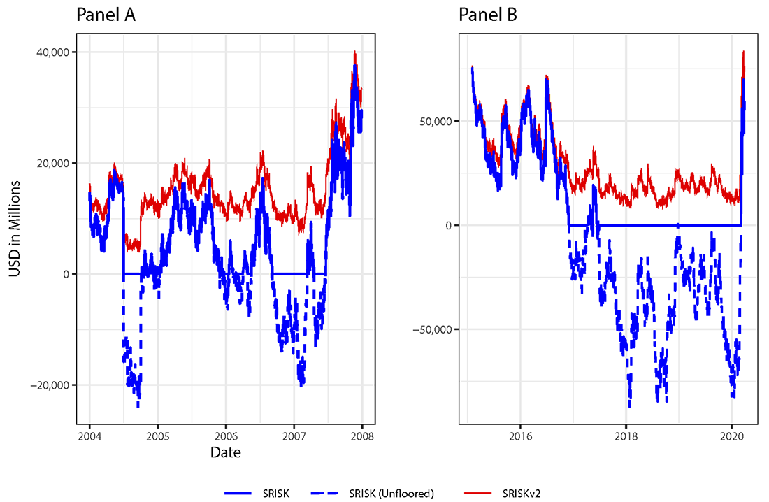
Between the summer of 2005 and the summer of 2007, the SRISKv2 of JPMC fluctuates between $10 Bln and $20 Bln. Meanwhile, SRISK is $0 for a large portion of this period. JPMC went on to receive a $25 Bln preferred stock investment from the Trouble Asset Relief Program (TARP) during the great financial crisis. A similar dynamic occurs between early 2017 and late 2019. SRISKv2 fluctuates between $10 Bln and $30 Bln during this period, while SRISK estimates that JPMC presents no systemic risk for almost that entire period.
This weakness in the calculation of SRISK affects how it ranks the systemic risk of firms, likely making the ranking less sensible. Table 1 compares SRISK and SRISKv2 for seven US GSIBs in July 31, 2019.5
Table 1: SRISK and SRISKv2 in July 31, 2019
| Bank | SRISK | SRISKv2 | Market Equity $Bln | Total Assets $Bln | ||
|---|---|---|---|---|---|---|
| $Bln | % of GSIBs | $Bln | % of GSIBs | |||
| JPMC | 0 | 0% | 17.3 | 14.4% | 376 | 2,727 |
| BAC | 0 | 0% | 14.4 | 12.0% | 286 | 2,396 |
| Citi | 46.6 | 66.6% | 47.3 | 39.4% | 161 | 1,988 |
| WFC | 0 | 0% | 14.6 | 12.2% | 214 | 1,923 |
| MS | 20.6 | 29.4% | 21.2 | 17.6% | 73.9 | 892 |
| BNYM | 0 | 0% | 1.9 | 1.6% | 44.2 | 381 |
| STT | 2.8 | 4.0% | 3.4 | 2.8% | 21.6 | 241 |
Brownlees and Engle (2016) propose that a firm's share of total SRISK may be a better measure of their systemic importance than their SRISK dollar amount. However, as this snapshot demonstrates, the share attributable to a firm under SRISK may be quite different from its share under SRISKv2. Under this example, SRISK attributes no systemic risk to four of the US GSIBs, including the two largest banks in the US by asset size, JPMC and BAC. Given its proper definition of capital shortfall, SRISKv2 improves upon SRISK in ranking firms' systemic importance and assigning their share of overall systemic risk.
Conclusion
This note sheds light on a conceptual flaw in SRISK and introduces a modified calculation that corrects this flaw. Given that SRISKv2 relies on a more conceptually sound definition of capital shortfall, we propose that academics and policymakers who wish to use the SRISK methodology to measure the systemic importance and vulnerability of firms rely instead on SRISKv2.
Appendix A – Calculating SRISKv2
The calculation of SRISKv2 follows closely the calculation of SRISK described in Brownlees and Engle (2016) except for how capital shortfall is calculated. The various calculation steps are described below.6
- To estimate SRISKv2 conditional on information up to period $$T$$, the first step is to estimate the joint dynamics of the return of firm $$i$$ and the market return using GARCH-DCC and data up to $$T$$.7 This estimation follows the methodology of Brownlees and Engle (2016). Specifically, return volatilities are modeled through the GJR-GARCH volatility model as follows (Glosten et al. 1993):
$$$$ \sigma_{i,t}^2 = \omega_{v_i} + \alpha_{v_i}r_{i,t-1}^2 + \gamma_{v_i}r_{i,t-1}^2 I^-_{i,t-1} + \beta_{v_i}\sigma_{i,t-1}^2 $$$$
$$$$ \sigma_{m,t}^2 = \omega_{v_m} + \alpha_{v_m}r_{m,t-1}^2 + \gamma_{v_m}r_{m,t-1}^2 I^-_{m,t-1} + \beta_{v_m}\sigma_{m,t-1}^2 $$$$
Where $$r_{i,t}$$ is the stock return of firm in period $$t$$; $$r_{m,t}$$ is the market return of firm in period $$t$$; $$\sigma_{i,t}^2$$ is the variance of the stock return of firm $$i$$ in period $$t$$; $$\sigma_{m,t}^2$$ is the variance of the market return in period $$t$$; $$I^-_{i,t-1}$$ is an indicator function that is equal to 1 if $$r_{i,t}$$ < 0 and 0 otherwise; and $$I^-_{m,t-1}$$ is an indicator function that is equal to 1 if $$r_{m,t}$$ < 0 and 0 otherwise. The indicator function component of these equations is meant to account for differences in volatility dynamics in response to negative returns. Research has shown that volatility increases more as result of negative returns (Rabemananjara and Zakoian 1993).
Under the DCC model (Engle 2002), the correlation between the volatility-adjusted return of firm $$i$$ ($$\epsilon_{i,t} = r_{i,t}/\sigma_{i,t}$$) and the volatility-adjusted market return ($$\epsilon_{m,t} = r_{m,t}/\sigma_{m,t}$$) is expressed as follows:
$$$$ Corr \begin{pmatrix} \epsilon_{i,t} \\ \epsilon_{m,t} \end{pmatrix} = \begin{bmatrix} 1 & \rho_{i,t} \\ \rho_{i,t} & 1 \end{bmatrix} = diag (Q_{i,t})^{-\frac{1}{2}} Q_{i,t} diag(Q_{i,t})^{-\frac{1}{2}} $$$$
where $$Q_{i,t}$$ is a pseudo correlation matrix. The DCC model specifies the dynamics of $$Q_{i,t}$$ as
$$$$Q_{i,t} = (1-\alpha_{Ci} - \beta_{Ci}) S_i + \alpha_{Ci} \begin{bmatrix} \epsilon_{i,t-1} \\ \epsilon_{m,t-1} \end{bmatrix} \begin{bmatrix} \epsilon_{i,t-1} \\ \epsilon_{m,t-1} \end{bmatrix}^{\prime} + \beta_{Ci}Q_{i,t-1} $$$$
Where $$S_i$$ is the unconditional correlation matrix of the volatility-adjusted return of firm $$i$$ and the volatility-adjusted market return.8 This translates to the following dynamic equation for $$\rho_{i,t}$$:
$$$$ \rho_{i,t} = \frac{(1-\alpha_{Ci} - \beta_{Ci}) \overline{\rho}_i + \alpha_{Ci}\epsilon_{i,t-1}\epsilon_{m,t-1} + \beta_{Ci}\rho_{i,t-1}}{\sqrt{1-\alpha_{Ci}(1-\epsilon_{m,t-1}^2)} \cdot \sqrt{1-\alpha_{Ci}(1-\epsilon_{i,t-1}^2)}} $$$$
Where $$\overline{\rho}_i$$ is the unconditional correlation of the volatility-adjusted return of firm $$i$$ and the volatility-adjusted market return.
B) Upon estimation of the GARCH-DCC model, we construct the standardized innovations for the market return and firm $$i$$'s return for the estimation sample period:9
$$$$ \epsilon_{m,t} = \frac{r_{m,t}}{\sigma_{m,t}} \text{ and } \xi_{i,t} = \left( \frac{r_{i,t}}{\sigma_{i,t}} - \rho_{i,t}\frac{r_{m,t}}{\sigma_{m,t}} \right) \Bigg/ \sqrt{1-\rho_{i,t}^2} $$$$
where $$t = 1, \dots, T$$. By construction $$\epsilon_{m,t}$$ and $$\xi_{i,t}$$ are zero mean, unit variance, uncorrelated with each other, and not serially correlated.
C) We simulate the value of capital shortfall ($$CS^{\prime}$$) for $$S$$ iterations.10 This step has the following sub-steps:
C.1) For each simulation iteration, we sample with replacement $$h$$ pairs of standardized innovations to create a pseudo sample of innovations from period $$T+1$$ to $$T+h$$.
$$$$ \begin{bmatrix} \xi_{i,T+t} \\ \epsilon_{m,T+t} \end{bmatrix}^s_{t=1,\dots,h} \text{ } s = 1, \dots, S $$$$
C.2) Using the pseudo sample of innovations as input to the GARCH-DCC dynamic equations for $$\sigma_{i,T+t}^2$$, $$\sigma_{m,T+t}^2$$, and $$\rho_{i,T+t}$$ described in step A and $$\sigma_{i,T}^2$$, $$\sigma_{m,T}^2$$, and $$\rho_{i,T}$$ as initial conditions, we generate logarithmic returns from period $$T+1$$ to period $$T+h$$.
$$$$ \begin{bmatrix} r_{i,T+t} \\ r_{m,T+t} \end{bmatrix}^s_{t=1,\dots,h} $$$$
C.3) Using the series of simulated daily returns, we calculate the arithmetic returns for firm $$i$$ and the market from period $$T$$ to period $$T+h$$.
$$$$ R^s_{i,T+1:T+h} = exp \left\{ \sum_{t=1}^h r^s_{i,T+t} \right\} - 1 $$$$
$$$$ R^s_{m,T+1:T+h} = exp \left\{ \sum_{t=1}^h r^s_{m,T+t} \right\} - 1 $$$$
C.4) Using $$R^s_{i,T+1:T+h}$$, we calculate the capital shortfall of firm $$i$$ at period $$T+h$$ in iteration $$s$$.
$$$$ CS^{\prime s}_{i,T+h} = max \left[ 0, kD_{i,T} - (1-k) W_{i,T} (1+R^s_{i,T+1:T+h}) \right] $$$$
Where $$D_{i,T}$$ is the book value of debt of firm $$i$$ at time $$T$$ (following Brownlees and Engle we assume that a firm's debt does not grow or shrink between $$T$$ and $$T+h$$).
D) After following the procedure described in step C for $$S$$ iterations, we calculate SRISKv2 as the average of $$CS^{\prime s}_{i,T+h}$$ conditional on $$R^s_{m,T+1:T+h}$$ being smaller than $$C$$.
$$$$ SRISKv2_{i,T} = \frac{ \sum_{s=1}^S CS^{\prime s}_{i,T+h} I \left\{R^s_{m,T+1:T+h} < C \right\} }{ \sum_{s=1}^S I\left\{R^s_{m,T+1:T+h} < C \right\} } $$$$
where $$I$$ is an indicator function.
References
Brownlees, Christian, and Robert Engle (2017). SRISK: A Conditional Capital Shortfall Measure of Systemic Risk. The Review of Financial Studies vol. 30 n. 1, 48-79.
Engle, Robert (2002). Dynamic Conditional Correlation: A Simple Class of Multivariate Generalized Autoregressive Conditional Heteroskedasticity Models. Journal of Business & Economic Statistics vol. 20 n. 3, 339-350.
Glosten, Lawrence R., Ravi Jagannathan, and David E. Runkle (1993). On the Relation between the Expected Value and the Volatility of the Nominal Excess Return on Stocks. The Journal of Finance vol. XLVIII n. 5, 1779-1801.
Rabemananjara, R., and Z. M. Zakoian (1993). Threshold Arch Models and Asymmetries in Volatility. Journal of Applied Econometrics vol. 8, 31-49.
1. The views expressed in this manuscript belong to the authors and do not represent official positions of the Federal Reserve Board or the Federal Reserve System. The authors thank Christian Brownlees for sharing the SRISK code and patiently explaining various details about its usage, and David Lynch and Ben Ranish for helpful comments and suggestions. Return to text
2. Quasi assets are equal to a firm's book value of debt plus its market value of equity. Return to text
3. Following Brownlees and Engle (2016), we use firm stock returns and market capitalization from CRSP and the book value of debt from COMPUSTAT. For the market return, we use the daily CRSP market value–weighted index return. Return to text
4. Brownlees and Engle (2016) assumed -10% and 22 days for $$C$$ and $$h$$, respectively. We assumed -20% and 120 days instead to highlight the potential for discrepancy between SRISK and SRISKv2. Return to text
5. Goldman Sachs was not included in this sample because its stock return data only becomes available post-1999, while we used data from October 30, 1986 to July 31, 2019 to estimate SRISK and SRISKv2 for the other firms. Return to text
6. The MATLAB code used to calculate SRISKv2 is available in https://github.com/marcomigueis/SRISKv2. Return to text
7. The SRISKv2 and SRISK estimates presented in this paper are based on an estimation sample period of October 30, 1986, to time $$T$$. Return to text
8. We estimate the GARCH-DCC model using the Oxford MFE Toolbox for MATLAB. See https://github.com/bashtage/mfe-toolbox/ retrieved on June 13, 2020. Return to text
9. Steps from B to C.3 follow the simulation methodology described in Appendix A of Brownlees and Engle (2016). Return to text
10. In the SRISKv2 and SRISK calculations presented in the paper we used $$S$$ = 100,000. Return to text
Note: This note was updated on March 25, 2021, to correct a typo in the equation in Appendix section C.4.
Migueis, Marco, and Alexander Jiron (2020). "SRISKv2 - A Note," FEDS Notes. Washington: Board of Governors of the Federal Reserve System, September 18, 2020, https://doi.org/10.17016/2380-7172.2724.
Disclaimer: FEDS Notes are articles in which Board staff offer their own views and present analysis on a range of topics in economics and finance. These articles are shorter and less technically oriented than FEDS Working Papers and IFDP papers.