FEDS Notes
August 05, 2025
Wealth Heterogeneity and Consumer Spending
Samara Beach, William Gamber, and Patrick Moran
1. Introduction
Economists have become increasingly interested in the effects of household heterogeneity on macroeconomic dynamics.1 Changes in the distribution of income and wealth, coupled with advances in data and computation, have brought questions about how heterogeneity affects macroeconomic dynamics to the forefront of the discipline. Further, wealth has become increasingly concentrated among high-income households during recent decades, as seen across a variety of measures, including the Federal Reserve Board's Distributional Financial Accounts. In this note, we provide new evidence on the implications of wealth heterogeneity for consumer spending. In particular, we find that rising wealth concentration has reduced the average propensity to consume out of wealth, which helps to explain the weak recovery following the Great Recession.
The declining propensity to consume out of wealth that we document has important implications for our understanding of the macroeconomy, as it makes aggregate demand less responsive to fluctuations in asset prices and dampens the transmission of any policy interventions that affect household wealth. Further, we show that the declining propensity to consume out of wealth helps to explain the weak economic recovery following the Great Recession – a topic of considerable interest, with much attention given to the weak recovery in consumer spending (see e.g. Aladangady and Feiveson, 2018, Pistaferri, 2016). In particular, several studies have pointed to the role of household balance sheets in explaining the weak recovery (see e.g. Dynan, 2012; Mian et al., 2013).
In this note, we exploit data from the Distributional Financial Accounts to better understand how changes in the distribution of wealth affect aggregate consumer spending. In particular, we show that the propensity to spend out of wealth has declined over the past 20 years, and that this decline can be well-explained by changes in the distribution of wealth. Further, we find that these patterns can explain much of the weak economic recovery following the Great Recession. Adding wealth heterogeneity to our model allows us to explain nearly all of the slow recovery following the Great Recession. Our results imply that that changes in the distribution of wealth can have meaningful consequences for consumer spending.
2. The weak recovery in consumer spending
Our analysis builds on a puzzle put forward by Aladangady and Feiveson (2018) who showed that, while fluctuations in income and wealth perform well in explaining long-term trends in consumer spending prior to the Great Recession, this relationship has broken down in recent years, leading consumer spending to be persistently weak compared to fundamentals since the early 2010s. To demonstrate this puzzle, consider a simple linear model for real personal consumption expenditure $$C_t$$, with dependent variables real disposable personal income $$Y_t$$, government transfers $$T_t$$, and household wealth $$W_t$$:
$$$$ C_t=\alpha(Y_t -T_t) + \beta W_t + T_t + \epsilon_t.\ (1) $$$$
In this model, $$\alpha$$ represents the marginal propensity to consume out of non-transfer income and $$\beta$$ represents the propensity to consume out of wealth.2 Because consumption, wealth, and income are non-stationary, it is likely that $$\epsilon_t$$ exhibits heteroskedasticity. We therefore transform equation (1) to obtain an estimable equation that we can take to the data.3
$$$$ \frac{C_t-T_t}{Y_t-T_t}=\alpha+\beta\frac{W_t}{Y_t-T_t}+\ \widetilde{\epsilon_t}\ (2) $$$$
Figure 1 shows the predicted consumption-to-income ratio of this model in blue compared to the data in black. The figure shows that the model tracks the data quite well until around 2012, but diverges sharply thereafter, with the model predicting much stronger household spending than realized in the data. This is the sense in which we mean consumption was weak: average consumption was about 4-1/2 percent below what the historical relationship between consumption, income, and wealth would have predicted between 2012Q1 and 2019Q4. This is not just a historical issue. Indeed, Figure 1 shows that consumption continues to be weak relative to what fundamentals would suggest both during and after the pandemic.
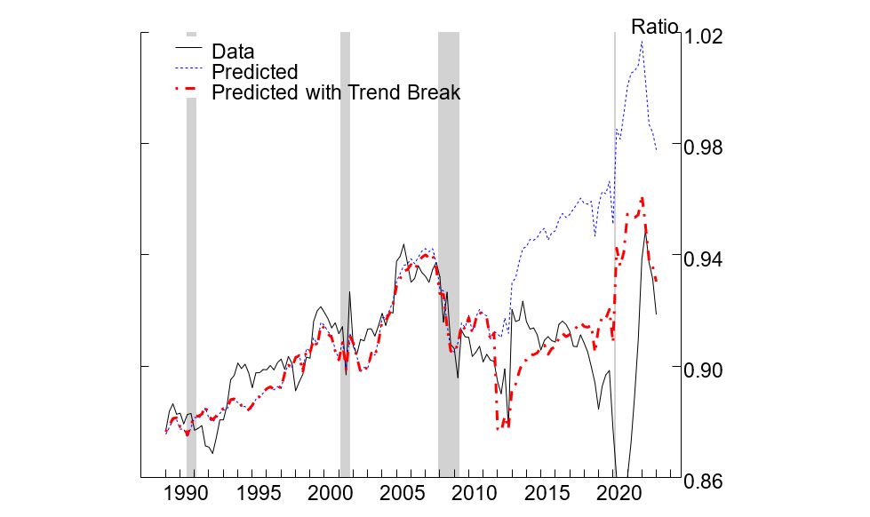
Note: Note that y-axis cuts off some observations in the "Data" series during 2020.
Source: U.S. Dept. of Commerce, Bureau of Economic Analysis; Financial Accounts of the United States, and authors' calculations.
In this note, we evaluate whether the changing distribution of wealth can explain the weak recovery in consumer spending following the Great Recession. We proceed as follows. First, we show that a declining propensity to consume out of wealth helps to resolve the discrepancy between our model predictions and observed consumer spending. Second, we evaluate to what extent increasing wealth concentration can explain the declining propensity to consume out of wealth. Third, we show that consumer spending is less sensitive to fluctuations in wealth held by high-income consumers, which is key to understanding the declining propensity to consume out of wealth during recent decades. Overall, we find that the rise in wealth during the past 15 years, much of which accrued to high-income households, did not translate into the same level of consumption as it would have if it had been more evenly distributed.
3. The declining propensity to spend out of wealth
The first column of Table 1 reports the estimated coefficients and standard errors of equation (2) estimated on quarterly data between 1964 and the end of 2011. The coefficient $$\beta$$, which denotes the marginal propensity to consume out of wealth, is around 3.5 cents per dollar, which is close to the estimates from studies that use panel data to estimate this coefficient, e.g. Chodorow-Reich et al. (2021). The coefficient $$\alpha$$ represents the MPC out of non-transfer income. This coefficient is 65 cents per dollar, which is in the range of recent micro-level estimates, such as Fagereng et al. (2021). As noted above, while this model provides a good fit of the data until the end of 2011, its out-of-sample fit has been much worse since then. Indeed, the out-of-sample root mean square error (RMSE) between 2012-2019 is more than four times larger than the in-sample RMSE between 1964-2011. Forecast errors were one-sided during this period, averaging 4 percent.4
Table 1: Baseline Model Estimate
| Dependent Variable: $$(C_t - T_t)/(Y_t - T_t)$$ |
||
|---|---|---|
| (1) | (2) | |
| Wealth-to-Income $$\beta$$ | 0.035*** | 0.033*** |
| (0.001) | (0.001) | |
| Trend Break (Post-2012) | -0.006*** | |
| (0.0004) | ||
| Constant $$\alpha$$ | 0.649*** | 0.659*** |
| (0.007) | (0.008) | |
| Observations | 191 | 222 |
| Adjusted $$R^2$$ | 0.824 | 0.784 |
| 1964 to 2011 RMSE | 0.0101 | 0.0101 |
| 2012 to 2019 RMSE | 0.0444 | 0.0149 |
| 1964 to 2011 Mean Error | -0.0001 | 0.0003 |
| 2012 to 2019 Mean Error | 0.0409 | -0.0007 |
Note: *p<0.1; **p<0.05; ***p<0.01
To improve model fit, we re-estimate equation (2) allowing for a time-varying propensity to spend out of wealth. There are two ways that we do this. First, we allow for a trend break in the coefficient on the wealth-to-income ratio. We choose to put the trend break in 2012, although the results would be similar even if the trend break were a few years earlier or later. Second, and even more flexibly, we allow for a time-varying propensity to spend out of wealth by re-estimating equation (2) using a rolling window on wealth. We choose a 10-year centered rolling window, where we allow the coefficient on wealth to vary while holding the other coefficient fixed at its estimated value.
The second column in Table 1 reports the estimates of the alternative model with a trend break in the propensity to spend out of wealth. We find that the trend break is statistically significant and implies that the MPC out of wealth has declined from 3.3 cents on the dollar before 2012, to 2.7 cents on the dollar post 2012, a decline of roughly 20 percent. Further, the declining propensity to consume out of wealth improves model fit substantially. The RMSE between 2012 and 2019 falls to 0.015 after including the trend break in the MPC out of wealth, a substantial improvement upon the model's previous performance, and the average residual is close to 0 over this period. Further, as shown in Figure 1, the predicted values of the model with the trend break (the dashed red line) obtain a much closer fit of the data (the solid black line) compared to the baseline model with a fixed MPC out of wealth (the dotted blue line). We find that the model with a rolling window obtains a similar improvement in model fit, although we omit the results for brevity.
Figure 2 reports the propensity to spend out of wealth coming from our two different models. The black dashed line shows the implied MPC out of wealth when we estimate equation (2) with a trend break, while the red line shows the implied MPC when we estimate equation (2) using a 10-year centered rolling window. The decline in the MPC is relatively similar regardless of whether we use the trend break or the rolling window. Further, the red line shows interesting variation over time. More specifically, we find that the MPC out of wealth was relatively stable around 3.3 to 3.4 cents on the dollar during the 1990s and early 2000s, but began to decline rapidly in the late 2000s, before eventually stabilizing at just under 2.7 cents on the dollar around 2016.
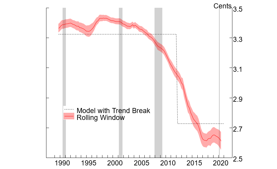
Source: U.S. Dept. of Commerce, Bureau of Economic Analysis; Financial Accounts of the United States, and authors' calculations.
To summarize, we find that allowing for a declining relationship between wealth and spending resolves much of the deviation between our model's fitted values and the observed spending data. This raises the natural question: what can explain the decline in the propensity to spend out of wealth during the late 2000s and early 2010s?
4. Rising wealth concentration
To answer this question, we turn to the Federal Reserve Board's Distributional Financial Accounts (DFAs), which provide quarterly estimates of disaggregated wealth holdings across the distribution of households, starting in 1989.5 Importantly for our use, the DFAs are consistent with the Federal Reserve's Financial Accounts (Z.1), so that aggregating across groups in the DFAs gives a time series equal to our definition of aggregate household wealth in equation (2). The DFAs report these estimates for several different measures of household heterogeneity; in this note, we focus on heterogeneity by income groups, which we ultimately found to be more important than heterogeneity by age or education groups.
Figure 3a shows the share of total net worth held by the top 20 percent of the income distribution between 1989 and 2024. The data show that wealth is more concentrated today than it was at the beginning of the DFA data, with the highest income quintile holding about 10 percentage points more wealth at the end of 2024 than they did in 1989:Q3, when the data began. There were particularly sharp increases in the share of wealth held by the top income quintile during the late 1990s, in the run-up to the Great Recession, and from around 2010–2015, after which wealth shares appear to have stabilized.6
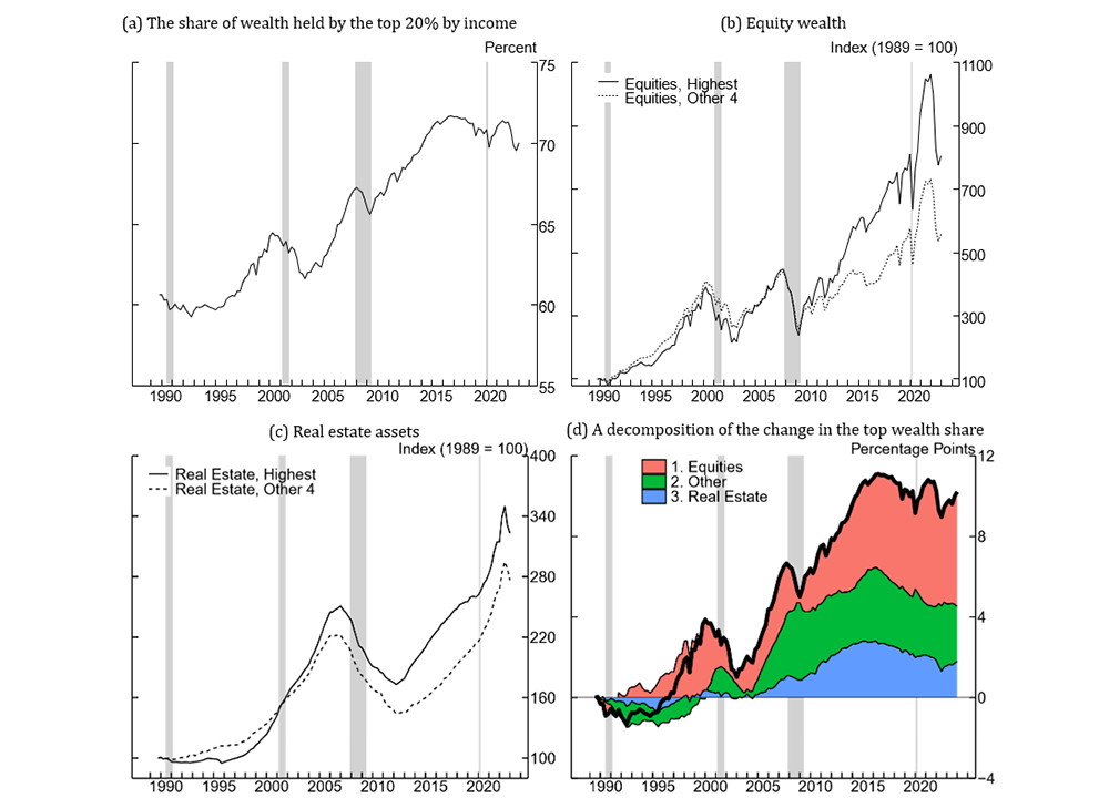
Notes: Panel (a) shows the share of nominal net worth held by the top 20 percent of households by income. Panels (b) and (c) show real asset holdings for the highest 20 percent of households by income and the bottom 80 percent of households by income. These series are indexed to 100 in 1983:Q3, the first observation of the DFA series. We deflate using the PCE deflator: Panel (d) shows a decomposition of the change in the share of wealth held by the top 20 percent of income into its contributions from three subcomponents. Key identifies in order from top to bottom.
Source: Federal Reserve, Distributional Financial Accounts of the United States.
Figures 3b and 3c show the paths of real asset holdings in equities and real estate, for these two income groups, where we normalize asset holdings to be 100 in 1989:Q3. The figure shows that equity and real estate holdings grew similarly for high-income households as for the remaining households during the 1990s and early 2000s.7 That said, the paths of asset holdings diverged starting in the late 2000s, roughly around the time of the recovery from the Great Recession. After then, equity wealth for the top income group grew at a much faster pace than for the remaining households. And, while real estate wealth generally grew at a slower rate than overall wealth, the highest-income households fared better than lower-income households.
Which types of assets contributed most to the rise in wealth concentration? Figure 3d shows a decomposition of the change in wealth shares since 1989 across the different asset classes we consider.8 The figure shows that equity wealth accounts for much of the rise in wealth concentration, with a smaller additional boost from real estate. In addition, equities account for almost all of the continued rise in wealth concentration since 2009.9
The patterns documented in these charts suggest a potential explanation for the declining MPC out of wealth. Wealth gains after the Great Recession accrued disproportionately to higher-income households, whose propensity to consume may be lower, for instance due to less-binding credit constraints or a diminishing marginal utility of consumption, which is a hallmark of essentially all economic models. In the next section, after obtaining new estimates on heterogeneity in the MPC out of wealth across the income distribution, we demonstrate that this explanation can quantitatively account for the declining MPC out of wealth.
5. The distribution of wealth and consumer spending
To assess heterogeneity in the propensity to consume out of wealth held by different segments of the income distribution, we develop a model of consumer spending that explicitly accounts for wealth heterogeneity. More specifically, we alter equation (2) to decompose aggregate household wealth into two parts: (i) wealth held by the top 20 percent of the income distribution and (ii) wealth held by the bottom 80 percent of the income distribution.10 We then include both components of aggregate wealth in our simple time-series model relating consumption to income and wealth:
$$$$ \frac{C_t-T_t}{Y_t-T_t}=\alpha+\beta^{TopQuintile}\frac{W_t^{TopQuintile}}{Y_t-T_t}+\beta^{Bottom4}\frac{W_t^{Bottom4}}{Y_t-T_t}+\epsilon_t\ (3) $$$$
Of course, there are a number of alternative ways that we could have added heterogeneity to our baseline forecasting model. We decided to focus on wealth held by different segments of the income distribution due to the fact that these measures show such a stark increase in concentration during the past 25 years, as shown in Figure 3a. While we also experimented with alternative specifications that included wealth held by different age and education groups, we ultimately found that heterogeneity along these other dimensions was less important in explaining consumer spending than the one that we study in this note.
Table 2 reports the coefficients and standard errors estimated based on equation (3). We find meaningful differences in the propensity to consume out of wealth held by different segments of the income distribution. In particular, fluctuations in wealth held by the top 20 percent of the income distribution imply an increase in spending of 0.8 cents on the dollar, which is substantially less than the aggregate propensity to consume out of wealth of roughly 3.3 to 3.5 cents on the dollar, which we reported in Table 1. In contrast, fluctuations in wealth held by the bottom 80 percent of the income distribution imply an increase in spending of roughly 7.5 cents on the dollar, much larger than the aggregate MPC estimate. While our estimate of 7.5 cents on the dollar is relatively large, it's important to note that the wealth-weighted-average MPC out of wealth remains remarkably similar to the aggregate MPC out of wealth reported in Table 1. Further, the qualitative patterns that we recover are consistent with a large theoretical and empirical literature finding that households who are less credit-constrained have a lower MPC (see e.g. Fagereng et al., 2021).
Table 2: Heterogeneity in the Propensity to Consume out of Wealth
| Dependent Variable: $$\frac{C_t-Y_t}{Y_t-T_t}$$ |
|
|---|---|
| Top Quintile Wealth | 0.008*** |
| (0.001) | |
| Other Quintiles' Wealth | 0.075*** |
| (0.008) | |
| Constant | 0.662*** |
| (0.023) | |
| Observations | 119 |
| Adjusted $$R^2$$ | 0.597 |
| 1989 to 2011 RMSE | 0.0103 |
| 2012 to 2019 RMSE | 0.0146 |
| 1989 to 2011 Mean Error | -0.0012 |
| 2012 to 2019 Mean Error | 0.005 |
Note: *p<0.1; **p<0.05; ***p<0.01
5.1. Explaining the declining propensity to spend out of wealth
To what extent does the rising concentration of wealth help to explain the declining propensity to consume out of wealth? To answer this question, we compute a time-varying aggregate MPC out of wealth that explicitly accounts for trends in the concentration of wealth. This is performed by combining equations (2) and (3). As a result, the aggregate MPC is simply the wealth-share-weighted average of the MPCs that we estimated for each income group:
$$$$ \beta_t=\frac{W_t^{TopQuintile}}{W_t}\beta^{TopQuintile}+\frac{W_t^{Bottom4}}{W_t}\ \beta^{Bottom4}\ (4) $$$$
This calculation yields a time-varying MPC $$\beta_t$$, which declines as the share of wealth owned by the top 20 percent of the income distribution increases, due to the fact that we estimate $$\beta^{TopQuintile}$$ < $$\beta^{Bottom4}$$.
Figure 4a reports our estimates of the time-varying MPC out of wealth, where the solid blue line shows our estimate of $$\beta_t$$ computed using our model with wealth heterogeneity. We find that the time-varying MPC out of wealth implied by our model with wealth heterogeneity closely tracks the aggregate MPC implied by the rolling window (the solid red line) and the post-2012 trend break (the black dashed line). In particular, adding wealth heterogeneity into our model allows us to explain roughly 94 percent of the decline in the MPC in the rolling window model from 1989Q3 to 2019Q4. As a result, we conclude that extending our model to explicitly account for wealth heterogeneity allows us to closely replicate the empirical evidence on the declining propensity to spend out of wealth.
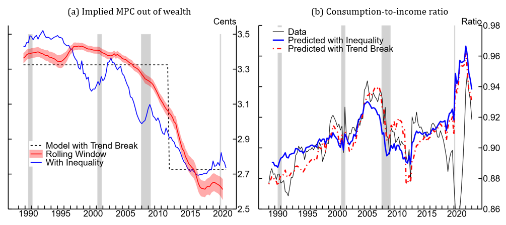
Source: U.S. Dept. of Commerce, Bureau of Economic Analysis; Federal Reserve, Financial Accounts of the United States; Federal Reserve, Distributional Financial Accounts, and authors' calculations.
5.2. Explaining the slow recovery in consumer spending
To what extent does the above-documented heterogeneity in wealth help to explain the slow recovery in consumer spending following the Great Recession, which we previously reported in Figure 1? To answer this question, we forecast consumer spending using equation (3), now allowing for heterogeneity in the propensity to spend out of wealth for different income groups. This model allows us to predict consumer spending while explicitly accounting for wealth heterogeneity.
Figure 4b shows the predicted consumption-to-income ratio coming from our model with wealth heterogeneity (the thick blue line). We find that the consumption forecast coming from the model with wealth heterogeneity closely tracks the forecast coming from the model with a trend break (the dashed red line) and thus obtains a significantly closer fit of the data (the black line) relative to the initial model without wealth heterogeneity or a time-varying propensity to consume out of wealth. Indeed, model fit improves substantially compared to the baseline model forecast shown in blue in Figure 1, which predicted much higher consumer spending than was ultimately realized in the data.
As a result, forecast errors are greatly reduced when we add wealth heterogeneity into our model of consumer spending. Table 2 shows that the RMSE between 2012-2019 is 0.015 in our model with wealth heterogeneity, almost identical to the model with the trend break, and a substantial improvement upon our baseline model with a time-invariant MPC out of wealth, which delivered an RMSE of 0.044 (Table 1).
Overall, while we do not seek to rule out all potential alternative explanations, we find that accounting for wealth heterogeneity significantly improves our model's ability to explain observed spending data. We find that adding wealth heterogeneity to our model allows us to explain roughly 88.7 percent of the slow recovery in consumer spending following the Great Recession, computed based on the average gap between predicted and actual spending from 2012Q1 to 2019Q4. As a result, we conclude that wealth heterogeneity goes a long way in accounting for the slow recovery in consumer spending.
5.3. Alternative hypothesis: heterogeneity across wealth categories
Before wrapping up, we evaluate the sensitivity of our results to an alternative hypothesis for the declining propensity to consume out of wealth and the weak recovery in consumer spending. In particular, to what extent might these findings be driven by changes in the composition of wealth across different categories (e.g. housing, equities, etc.) rather than changes in who owns those assets?
As discussed previously, equities were an important factor driving the rise in wealth concentration among top income households in the U.S. Indeed, there have been large movements in the composition of wealth over time, as shown in Figure 3. One potential alternative explanation for the declining MPC out of wealth could be that wealth has shifted to lower-MPC categories over time, causing the average MPC to fall. In this section we assess this alternative hypothesis. Ultimately we conclude that the concentration of wealth is more important than the composition of wealth when it comes to accounting for the declining propensity to spend out of wealth and the slow recovery following the Great Recession.
To test the above hypothesis, we estimate an equation analogous to equation (3), but decomposing net wealth into three broad categories: equities, real estate, and other. The whiskered dots in the left panel of Figure 5 show the estimated MPCs for each category. The figure shows that the MPC out of equity wealth is less than one quarter of the MPC out of real estate wealth. We estimate an MPC out of housing wealth of just over 5.0 cents on the dollar, which is consistent with previous estimates.11In contrast, the MPC out of equity wealth is only slightly above 1.0 cent on the dollar. The MPC out of 'other wealth' falls roughly in between the MPCs of equity and real estate.
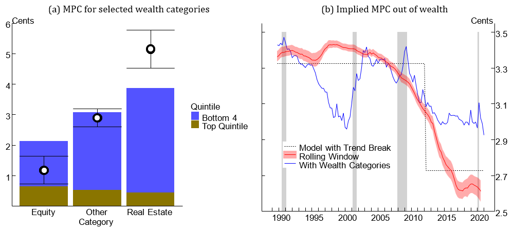
Notes: Whiskered dots in panel (a) show the estimates of MPCs for three categories of net worth. The sum of each of the stacked bars shows the predicted MPC for each asset category using information about the differences in asset holdings across income groups, as well as differences in MPCs across income groups. Key identifies in order from top to bottom. The blue line in panel (b) shows the time-varying MPC implied by our estimates of category-specific MPCs (shown in the whiskered dots in panel (a)) and the time-varying share of wealth in each category.
Source: U.S. Dept. of Commerce, Bureau of Economic Analysis; Distributional Financial Accounts of the United States, and authors' calculations.
We then combine our MPC estimates with the share of wealth held in each category to recover a time-varying aggregate MPC, using an approach similar to equation 4. The right panel of Figure 5 shows this MPC in solid blue. Based on changes across wealth categories alone, this model predicts a decline in the MPC out of wealth in the late 1990s, inconsistent with the previous empirical evidence coming from the rolling window model. Moreover, although this model predicts some decline in the MPC out of wealth in the 2010s, as the share of wealth in equities rose, the decline is smaller than estimated previously. Ultimately, the rise in equity wealth during this period primarily accrued to high-income households, who have lower MPCs. As a result, we conclude that our model of wealth heterogeneity performs better over this period.
In fact, we find that differences in MPCs between income groups helps to explain the differences in MPCs that we estimate between wealth categories. To show this, we impute an MPC for each wealth category based on what we know about the MPCs for each income group, as well as their wealth holdings. Specifically, for each wealth category $$j$$, we compute this imputed MPC by averaging our two income groups' MPCs, weighted by each group's holdings of that particular asset category, shown in equation 5. (Recall that our estimate of the MPC for the top quintile is 0.8 cents per dollar, while for the other quintiles it is 7.5 cents per dollar.)
$$$$ \widehat{MPC_j}=\left(0.8\ cents\right)\times\frac{Top\ quintile's\ holdings\ of\ category\ j}{Total\ wealth\ in\ category\ j}\ $$$$
$$$$ +\left(7.5\ cents\right)\times\frac{Bottom\ 4\ quintiles'\ holdings\ of\ category\ j}{Total\ wealth\ in\ category\ j}\ (5) $$$$
We show the imputed MPCs in the stacked bars shown in the left panel of Figure 5. The height of each combined bar shows the imputed MPC out of wealth for each wealth category $$\widehat{MPC_j}$$, while the shaded bars show the contribution coming from each income group. This imputed MPC captures the fact that lower-income households' portfolios are tilted more toward real estate than equities, and the opposite holds for the top quintile of the income distribution. As this figure shows, the difference between the estimated MPCs (whiskered dots) for real estate and equity is roughly four cents, and the difference between the imputed MPCs (stacked bars) for these two categories is almost two cents. So, our imputation can account for almost half of the estimated difference between MPCs for equity compared to real estate. In other words, equity wealth appears to have a lower MPC in part because it is disproportionately held by higher-income households, who have a lower MPC.12
6. Conclusion
In this note, we demonstrate using a parsimonious time-series model that changes in the distribution of wealth help to explain the declining propensity to consume out of wealth during recent decades. Further, we show that this phenomenon helps to explain the weak recovery in household spending after the Great Recession and the continuing persistent weakness in spending relative to what would be suggested by the historical relationship between consumption, income, and wealth.
We view this note as contributing to a large and growing literature in macroeconomics that seeks to assess the effects of heterogeneity on macroeconomic dynamics.13We show in a simple time series model that the rising concentration of wealth led the MPC out of wealth to decline and quantitatively accounts for the weak recovery in spending after the Great Recession. Future work could investigate this hypothesis further using more detailed microdata or a structural model. However, we view this note as a simple exposition of how one particular form of heterogeneity can affect macroeconomic dynamics in a significant way.
Our findings on the relationship between wealth heterogeneity and consumer spending may have important implications for policymakers and forecasters. In particular, our results suggest that asset price growth over the past 5 years may have disproportionately supported the spending of high-income households, consistent with recent empirical evidence on consumer spending across the distribution (Chylak et al., 2024). Looking forward, the muted sensitivity of spending to wealth also suggests that fluctuations in equity and house prices now translate into smaller movements in consumption and GDP than they used to, thus dampening one of the key channels through which aggregate shocks and monetary policy decisions can affect the macroeconomy.
References
Aladangady, Aditya, "Housing wealth and consumption: Evidence from geographically linked microdata," American Economic Review, 2017, 107 (11), 3415–3446.
_ and Laura Feiveson, "A Not-So-Great Recovery in Consumption : What is Holding Back Household Spending?," FEDS Notes 2018-03-08, Board of Governors of the Federal Reserve System (U.S.) March 2018.
Batty, Michael M., Joseph S. Briggs, Alice Henriques Volz, Karen M. Pence, and Paul A. Smith, "The Distributional Financial Accounts," FEDS Notes 2019-08-30, Board of Governors of the Federal Reserve System (U.S.) August 2019.
Chodorow-Reich, Gabriel, Plamen T. Nenov, and Alp Simsek, "Stock Market Wealth and the Real Economy: A Local Labor Market Approach," American Economic Review, May 2021, 111 (5), 1613–1657.
Chylak, Jack, Leo Feler, and Sinem Hacioglu Hoke, "A Better Way of Understanding the US Consumer: Decomposing Retail Sales by Household Income," FEDS Notes 2024-10-11, Board of Governors of the Federal Reserve System (U.S.) October 2024.
Dynan, Karen, "Is a Household Debt Overhang Holding Back Consumption," Brookings Papers on Economic Activity, 2012, 43 (1 (Spring), 299–362.
Fagereng, Andreas, Martin B. Holm, and Gisle J. Natvik, "MPC Heterogeneity and Household Balance Sheets," American Economic Journal: Macroeconomics, October 2021, 13 (4), 1–54.
Hubmer, Joachim, Per Krusell, and Anthony A. Smith., "Sources of US Wealth Inequality: Past, Present, and Future," NBER Macroeconomics Annual, 2021, 35, 391–455.
Kaplan, Greg and Giovanni L. Violante, "Microeconomic Heterogeneity and Macroeconomic Shocks," Journal of Economic Perspectives, August 2018, 32 (3), 167–94.
Mian, Atif, Kamalesh Rao, and Amir Sufi, "Household Balance Sheets, Consumption, and the Economic Slump*," The Quarterly Journal of Economics, 09 2013, 128 (4), 1687–1726.
Pistaferri, Luigi, "Why Has Consumption Remained Moderate after the Great Recession?," Mimeo, Stanford University October 2016.
Stock, James H and Mark W Watson, "A Simple Estimator of Cointegrating Vectors in Higher Order Integrated Systems," Econometrica, July 1993, 61 (4), 783–820.
1. See for instance Janet Yellen's 2016 speech on "Macroeconomic Research After the Crisis" where she states "I am glad to now see a greater emphasis on the possible macroeconomic consequences of heterogeneity." Return to text
2. We assume a linear relationship for simplicity, although, as we show, this relationship generally captures much of the long-run variation in consumer spending before 2012. Further, we assume that households spend all of their transfer income. For most periods, this is likely to be a reasonable assumption, as transfers tend to be targeted to lower-income households with higher marginal propensities to consume, and many transfers are in-kind (Fagereng et al., 2021). In practice, removing this restriction on the coefficient on transfer income generates an MPC near 1. Return to text
3. We estimate equation (2) on data between 1964Q3 and 2011Q4 using dynamic ordinary least squares (see Stock and Watson, 1993). The coefficient estimates are reported in Table 1. Return to text
4. The focus of this note is on the recovery from the Great Recession, and so we report forecast errors for a period ending before the 2020 recession. That said, as shown in the blue dotted line in Figure 1, a model using the pre-2012 MPC out of wealth also predicts much higher consumption after 2020. Return to text
5. For more details on the methodology behind the DFAs, see: Batty et al. (2019) Return to text
6. In this note, we treat changes in the distribution of wealth as exogenous. As Hubmer et al. (2021) show, changes in the tax code were a central contributor to the rise in wealth concentration. Return to text
7. An income-group's equity holdings are defined here as the sum of the DFA-provided series "corporate equities and mutual fund shares" and "defined contribution pension entitlements", based on the formula for series LA153064475.Q from the Z.1 financial accounts. Return to text
8. Each line shows a counterfactual path of the share of wealth held by the top 20 percent of the income distribution in which we allow one component of wealth to vary as it did in the data and distribute all remaining net worth according to its share in 1989:Q3. Return to text
9. We also show the contribution from net worth excluding real estate and equities, which we denote by "other wealth." This category includes assets such as bank deposits, durable goods, pensions, as well as liabilities, including mortgages and consumer credit. Return to text
10. We focus on the top 20 percent of the income distribution given its salience and given that this segment of the population holds such a considerable share of wealth. Reassuringly, we find relatively similar results if we instead focus on the top 5 or top 1 percent of the distribution. We again use dynamic OLS to estimate this regression. Return to text
11. For further evidence on the MPC out of housing wealth, see Aladangady (2017), who finds an MPC out of housing wealth of 4.7 cents on the dollar for homeowners and zero for non homeowners, consistent with our results. Return to text
12. As noted, this mechanism can only explain about half of the difference between our estimates of the MPC for equity and real estate. Other mechanisms could drive the remaining difference between these MPCs, including different transaction costs or a difference in the persistence of returns. Return to text
13. Citations are too numerous to include here. However, see Kaplan and Violante (2018) for a discussion of some of this work. Return to text
Beach, Samara, William Gamber, and Patrick Moran (2025). "Wealth Heterogeneity and Consumer Spending," FEDS Notes. Washington: Board of Governors of the Federal Reserve System, August 05, 2025, https://doi.org/10.17016/2380-7172.3838.
Disclaimer: FEDS Notes are articles in which Board staff offer their own views and present analysis on a range of topics in economics and finance. These articles are shorter and less technically oriented than FEDS Working Papers and IFDP papers.