FEDS Notes
December 29, 2020
Why Were Treasury Yields So Stable Over the Summer?
Kasper Joergensen and Laura Wilcox
Early this year, economic activity plummeted as COVID-19 cases around the world surged and governments enacted restrictions to mitigate the spread of the virus. Over the summer, as restrictions were gradually lifted, the near-term outlook for the economy improved and economic data prints began to come in stronger than expected. For example, the Citigroup Economic Surprise Index reached all-time highs in July, reflecting that economic indicators were well above expectations (figure 1). Although medium- and long-term Treasury yields typically rise when the near-term economic outlook improves, Treasury yields remained unusually stable, fluctuating only in narrow ranges (figure 2).1 In this Note, we discuss factors that have likely contributed to the stability of yields over the summer and early fall. We argue that the large gap between current economic conditions and the FOMC's monetary policy goals, together with monetary policy currently being at the effective lower bound, has been an important factor contributing to the low volatility of yields. That said, another contributing factor could be that the signal embedded in recent data releases about the economic outlook has arguably been weaker than normal, which has likely dampened the reaction of yields to economic data surprises.
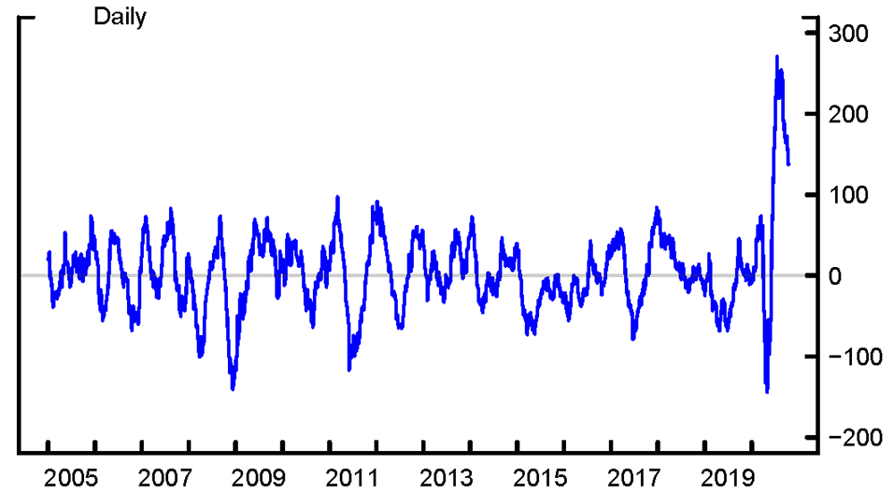
Note: Measures whether economic indicators are above or below consensus forecasts.
Source: Bloomberg Finance LP, Bloomberg Terminals (Open, Anywhere, and Disaster Recovery Licenses).
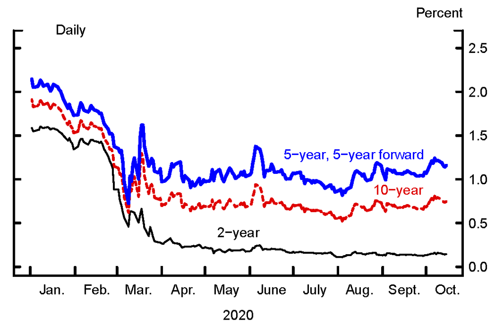
Source: Board staff calculations.
Factors contributing to the stability of Treasury yields
The gap between current economic conditions and the FOMC's monetary policy goals of maximum employment and price stability pins the policy rate at the effective lower bound. Current economic conditions likely warrant an expected policy rate path that, absent the lower-bound constraint, would be substantially negative over the next few years. As a result, the observable expected policy rate path over the next few years is relatively unresponsive to changes in the near-term economic outlook, because it is constrained by the effective lower bound. The FOMC's forward guidance may have also reinforced the view that current economic conditions are far from those associated with liftoff.2 In figure 3, we plot the expected policy rate path, implied by OIS quotes and unadjusted for term premiums, at the end of the first three quarters of 2020. Consistent with the expected policy path being unresponsive to changes in the near-term economic outlook, the OIS-implied policy path over the next few years remained flat and stable near the effective lower bound over the summer and early fall. The median respondent to the Federal Reserve Bank of New York's Survey of Primary Dealers (the "Desk survey") has likewise reported a flat path at the effective lower bound for the next few years as the expected modal outcome. This stability of the policy path has likely passed through to medium-term Treasury yields as well.
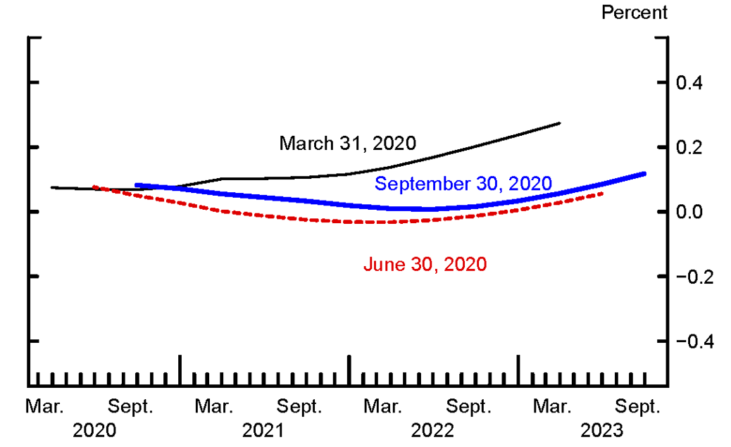
Note: The path is estimated using overnight index swap quotes with a spline approach and a term premium of 0 basis points.
Source: Bloomberg Finance LP, Bloomberg Per Security Data License; Board staff calculations.
That said, it is notable that forward rates well beyond the expected liftoff horizon, including the five-year, five-year forward rate in figure 2, have also remained stable.3 While longer-term forward rates are at historically low levels, they are still above their effective lower bound. The historically low levels of longer-term forward rates may have reduced the sensitivity to weaker-than-expected data somewhat, but it is not clear that proximity to the lower bound should have reduced their sensitivity to positive economic data surprises much. Indeed, one might have expected these forward rates to exhibit sensitivity to data surprises, in part through responses in the term premium components of long-horizon forward rates. But the net effect of, for example, the June through September employment report releases on the five-year, five-year forward rate, as measured by the cumulative change in narrow windows around each release, was only about 5 basis points. The reaction of equity prices (which are also not constrained by the effective lower bound) was similarly muted. Thus, other factors than monetary policy being pinned at its lower bound have likely contributed to the stability of Treasury yields.
Another factor contributing to the limited fluctuations of both medium- and longer-term yields may have been a weaker signal in recent data releases. The surprise component in a data release is typically measured as the deviation of the realized data print from the average or median of survey respondents' modal expectations. However, the global pandemic has caused considerable uncertainty about the economic outlook, particularly for the labor market, so market participants may have had little conviction about their modal expectations for this summer's data releases. For this reason, market participants may have taken a much weaker signal about the economic outlook from the large data surprises, leading long-term yields and forward rates to seem less responsive to news.
Measuring the signal from data surprises in certain and uncertain times
The surprise component in a data release is typically measured as the deviation from the average or median of survey respondents' modal expectations. This measure is then typically standardized by dividing the data surprise by the historical standard deviation of past data surprises to adjust for forecast uncertainty. For example, the Citi Economic Surprise Index takes this measure as an input. Adjusting for forecast uncertainty is desirable because if forecasters have little conviction in their modal expectation even fairly large deviations from expectations may not be particularly surprising. But the historical standard deviation of surprises may, at times, not be an adequate measure of uncertainty about expectations. For example, the COVID-19 pandemic has brought considerable uncertainty about the economic outlook, which likely means forecasters have had much less conviction about their modal expectations for this summer's data releases than they do normally. Consistent with low conviction about expected outcomes of recent data releases, survey responses from Action Economics reveal elevated dispersion among forecasters, measured as the cross-sectional standard deviation of survey respondents reported expectations, in recent months. Although survey dispersion is not strictly the same as uncertainty, it is a typical proxy; see e.g. Rich, Raymond, and Butler (1992). Using dispersion as a proxy for uncertainty, the largest data surprises have also been the releases for which forecast uncertainty was the highest. For the labor market, large surprises for nonfarm payrolls and unemployment insurance initial claims were accompanied by record-high dispersion among forecasters (the left and middle panels in figure 4). In contrast, CPI data releases resulted in smaller surprises and showed only a modest uptick in dispersion among forecasters (the right panel in figure 4).
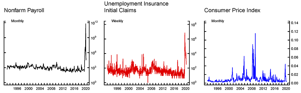
Note: Survey dispersion is calculated as the cross−sectional variance of survey respondents' reported expectations. The left panel measures the net change in total nonfarm employment since the previous month; the y−axis is plotted on a logarithmic scale. The middle panel measures the new unemployment insurance initial claims since the previous week; the y−axis is plotted on a logarithmic scale. The right panel measures the monthly percentage change in the consumer price index.
Source: Action Economics, LLC, Action Economics Weekly Survey, http://www.actioneconomics.com/index.php.
We therefore "standardize" the economic data release surprises by survey dispersion to produce a "dispersion-adjusted" data surprise measure. This measure allows us to check if the response of long-term yields to economic data releases has been anomalously small while accounting for the vast uncertainty surrounding the economic outlook in recent months.
Several other measures of uncertainty exist: stock market volatility measures (e.g. the VIX), newspaper-based measures (Baker, Bloom, and Davis, 2016), or statistical uncertainty measures (e.g. Engle, 1982; Bollerslev, 1986; Jurado, Ludvigson, and Ng, 2015). These measures are mostly broad uncertainty indexes and do not distinguish between, say, labor market and inflation uncertainties. The exception is conditional volatility estimates from GARCH-type models, which we can compute for each data surprise series. We have found that survey dispersion and GARCH-based measures of surprise uncertainty generally are positively correlated. For example, for nonfarm payrolls and unemployment insurance claims, we compute a correlation of the order of 0.5 to 0.8.4 For our application, the advantage of the Action Economics survey dispersion is that it is tailored to each data release and that it is forward looking (unlike statistical uncertainty measures, which require extrapolation based on historical correlations in the data).
Evidence from employment report releases
In order to compute expected responses of yields to employment report releases, consider the typical event-study regression
$$$$ \Delta y_t^{(n)} = \alpha + \beta X_t + \varepsilon_t, $$$$
Where $$ \Delta y_t^{(n)} $$ denotes the change in a n-year yield in a tight window around a data release, $$X_t$$ measures the surprise component of the release, and $$ \varepsilon_t $$ is a residual. This type of regression is used in e.g. Gürkaynak, Sack, and Swanson (2005), among many others. We estimate two versions of the event study regression outlined above for the 10-year Treasury yield, using a 30 minute (5 minutes before, 25 minutes after) event window, on the sample January 1993 through December 2019. The first version uses the standard data surprise measure, while the second version uses our dispersion-adjusted measure. Our right-hand-side variables are surprises in nonfarm payrolls, hourly earnings, and the unemployment rate. We calculate residuals for both versions of the regression and standardize the out-of-sample residuals for 2020 by the estimated standard deviation of in-sample residuals for 1993 through 2019. Standardized out-of-sample residuals may then be considered anomalous if they are numerically large. Assuming residuals are normally distributed, out-of-sample residuals should exceed 1.96 numerically only five percent of the time, making it a natural threshold.
Figure 5 plots the standardized residuals. The shaded region marks the out-of-sample residuals for 2020. The left panel reports results based on the standard data surprise measure, while the right panel reports results based on our dispersion-adjusted measure. In the left panel, some out-of-sample residuals are more than 100 standard deviations below what we would have expected based on the standard event study model. In that case, we would interpret the yield as being unusually unresponsive to the release. However, the right panel shows that accounting for the vast uncertainty surrounding the release, as measured by the dispersion among forecasters, overturns that result. The out-of-sample residuals are much smaller and all fall in the region that we would have expected based on the dispersion-adjusted model.
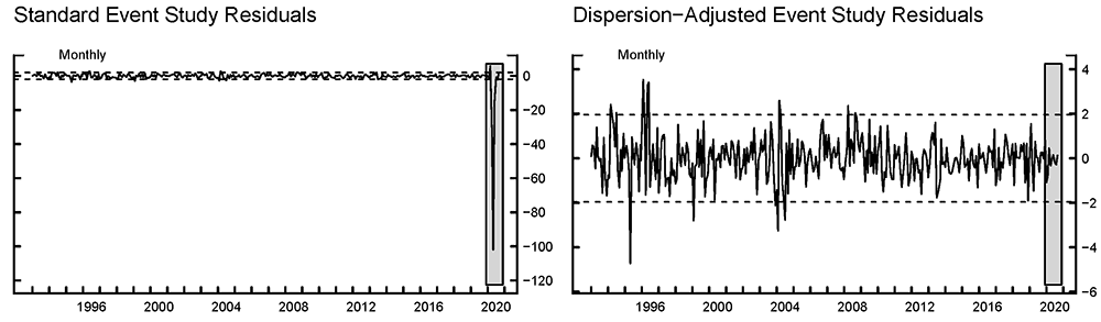
Note: The standardized residuals are calculated from employment report event study regressions using a 30 minute window around (5 minutes before and 25 minutes after) the release. Shading denotes observations from 2020.
Source: Action Economics, LLC, Action Economics Weekly Survey, http://www.actioneconomics.com/index.php; Bloomberg Finance LP, Bloomberg Per Security Data License.
Swanson and Williams (2014) interpret yields that are unusually unresponsive to a broad set of data releases as being constrained by the effective lower bound, suggesting there is less scope for monetary policy to affect such constrained yields. They found that, during the period when monetary policy was last at the effective lower bound, yields in the 5- to 10-year segment of the curve were largely unconstrained. While we might be led to conclude that the 10-year yield is currently constrained based on the standard data surprise measure, adjusting for the weak signal in recent data releases reveals that yields have exhibited about expected responsiveness to economic news. One caveat to this result could be that it hinges solely on responses to a few monthly employment reports. However, in unreported results, we have found similar results for unemployment insurance initial claims and CPI data releases.
Concluding remarks
The large gap between current economic conditions and the FOMC's monetary policy goals, together with monetary policy being at the effective lower bound, has likely contributed to relatively low volatility of Treasury yields over the summer and early fall. But other factors may have contributed to the stability as well. In particular, we find evidence that the weak signal in recent data releases about the economic outlook has dampened the reaction of both medium- and longer-term yields to economic data surprises.
References
Baker, S., N. Bloom, and S. J. Davis (2016). "Measuring Economic Policy Uncertainty." Quarterly Journal of Economics, vol. 134(4), pp. 1593-1636.
Bollerslev, T. (1986). "Generalized Autoregressive Conditional Heteroskedasticity." Journal of Econometrics, vol. 31(3), pp. 307-327.
Engle, R. F. (1982). "Autoregressive Conditional Heteroscedasticity with Estimates of the Variance of United Kingdom Inflation." Econometrica, vol. 50(4), pp. 987-1007.
Gürkaynak, R. S., B. Sack, and E. T. Swanson (2005). "The Sensitivity of Long-Term Interest Rates to Economic News: Evidence and Implications for Macroeconomic Models." American Economic Review, vol. 95(1), pp. 425-436.
Gürkaynak, R. S., B. Sack, and J. H. Wright (2007). "The U.S. Treasury Yield Curve: 1961 to the Present." Journal of Monetary Economics, Vol. 54(8), pp. 2291-2304.
Jurado, K., S. C. Ludvigson, and S. Ng (2015). "Measuring Uncertainty." American Economic Review, vol. 105(3), pp. 1177-1216.
Rich, R. W., J. E. Raymond, and J. S. Butler (1992). "The Relationship Between Forecast Dispersion and Forecast Uncertainty: Evidence From A Survey Data-ARCH Model." Journal of Applied Econometrics, vol. 7, pp. 131-148.
Swanson, E. T. and J. C. Williams (2014). "Measuring the Effect of the Zero Lower Bound on Medium- and Longer-Term Interest Rates." American Economic Review, vol. 104(10), pp. 3154-3185.
1. The yields and forward rates are from the Gürkaynak, Sack, and Wright (2007) data set. These data are available at https://www.federalreserve.gov/data/nominal-yield-curve.htm. Return to text
2. In its March, April, June, and July post-meeting statements, the FOMC communicated that it expected to maintain the target range of 0 to ¼ percent "until it is confident that the economy has weathered recent events and is on track to achieve its maximum employment and price stability goals." In the September post-meeting statement, this forward guidance became more explicit about the economic outcomes associated with liftoff, with the language being modified to "until labor market conditions have reached levels consistent with the Committee's assessments of maximum employment and inflation has risen to 2 percent and is on track to moderately exceed 2 percent for some time." The forward guidance language from September is consistent with the FOMC's newly updated Statement on Longer-Run Goals and Monetary Policy Strategy. Return to text
3. In the Desk's September surveys, the median respondent viewed the most likely timing of the first increase in the target range for the federal funds rate to be not until 2024. Return to text
4. The comparisons are based on GARCH(1,1) measures of conditional volatility computed from data surprises directly, i.e. from realized data prints minus median survey expectations from the Action Economics surveys. Return to text
Joergensen, Kasper, and Laura Wilcox (2020). "Why Were Treasury Yields So Stable Over the Summer?," FEDS Notes. Washington: Board of Governors of the Federal Reserve System, December 29, 2020, https://doi.org/10.17016/2380-7172.2824.
Disclaimer: FEDS Notes are articles in which Board staff offer their own views and present analysis on a range of topics in economics and finance. These articles are shorter and less technically oriented than FEDS Working Papers and IFDP papers.