FEDS Notes
May 12, 2023
Winners and losers from recent asset price changes
Edmund Crawley and William Gamber
Introduction
Asset prices and interest rates have changed dramatically and unexpectedly over the last two years as the Federal Reserve has raised its policy rate to combat higher inflation. In this note, we clarify the redistributive effects of these asset price changes in terms of welfare, which contrast sharply with those of wealth. Figure 1 depicts changes in the paths of six macroeconomic aggregates in the February 2023 CBO projection relative to their paths in the July 2021 projection.1 As shown in the figure, interest rates rose relative to expectations, inflation is higher than expected, house prices are higher than expected but are little changed in the long run, and equity prices are significantly lower than expected. In this note, we estimate the welfare effects of these asset price movements for people of different ages.
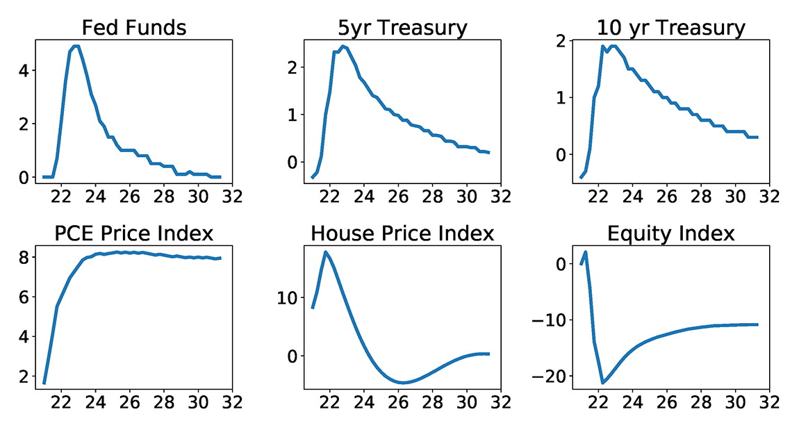
Note: Changes in the CBO projections from July 2021 to February 2023. Interest rate changes are in percentage points, index changes in percent. Panels are all nominal. Source: CBO and author calculations.
In our framework, a change in asset prices affects an individual's welfare only if they buy or sell the asset. Otherwise, the change in wealth implied by a change in the price of an asset is only "on paper." For example, a family who faces no financial constraints and lives in the same house for its entire life is not affected by changes in the value of that house.
We find that middle-aged individuals benefited significantly from these asset price movements, primarily driven by the decline in the price of equities. Retirees, on the other hand, were hurt by these asset price movements. These welfare results sharply contrast with the changes in wealth these groups have experienced: young people, whose few assets are concentrated in housing, have seen their wealth rise a little; people in middle age and older, who hold more equities than any other age group, have seen sharp declines in their wealth.
Methodology
We follow Fagereng et al (2022), who derive sufficient statistics for the first-order approximation of the welfare change due to asset price fluctuations. To implement these sufficient statistics in US data, we first extend them to cover long-term debt such as mortgages, including an adjustment for unexpected inflation. We then estimate the relevant components of these sufficient statistics using household microdata on asset holdings from the Survey of Consumer Finances (SCF) and long-term projections of asset prices constructed by the Congressional Budget Office.
Theoretical Framework
We are interested in quantifying the welfare changes due to fluctuations in asset prices. We compute these welfare changes in a model of households who maximize the discounted sum of future utility under expectations about the path of future economic outcomes. To express welfare in interpretable units, we estimate a "money metric" welfare measure. This measure answers the question: How much would a particular person (or group of people) pay for a given change in asset prices?
Fagereng et al (2022) derive closed form expressions for the first-order approximation of the money metric welfare gain associated with a particular path of asset prices, under some standard assumptions. For infinite maturity assets like equities and housing, this expression is:
$$$$ \Delta Welfare \approx \sum_{t=0}^{T} R^{-t} Net Sales_{t} \times Price Deviation_{t} $$$$
where Net Sales is an individual's net real sales of the asset, Price Deviation is the deviation of real prices from a counterfactual, and T is the last date at which the price deviates from its baseline.2 For assets with 1-period maturity, like short-term debt, this expression depends on asset holdings rather than net transactions3:
$$$$ \Delta Welfare \approx - \sum_{t=0}^{T} R^{-t} Debt Holdings_{t} \times Price Deviation_{t}. $$$$
Asset Holdings and Transactions
To implement these sufficient statistics, we need measures of both net sales and asset holdings. The SCF is a good source for data on asset holdings for households in the United States. However, the SCF is a repeated cross-sectional survey conducted every 3 years, and it does not contain direct information on asset purchases or sales. So, to impute net asset purchases, we follow the synthetic cohort methodology laid out in Feiveson and Sabelhaus (2019). This method relies on the following budget constraint to back out asset purchases between two consecutive waves of the SCF:
$$$$W_{c,t+3}=W_{c,t}^{survivors}+IFT_{c,(t,t+3)}+G_{c,(t,t+3)}+S_{c,(t,t+3)}$$$$
Where W denotes wealth, c denotes cohort and t and t+3 denote consecutive SCF waves. We adjust for the probability of death between consecutive waves, and the wealth of surviving individuals is denoted by $$W^{survivors}$$. IFT refers to inter-family transfers, either in the form of bequests or inter-vivos transfers, G are capital gains, and S denotes net asset purchases. We also convert household-level data to the individual level by allocating jointly-held assets equally. Given estimates of wealth, survival probabilities, inter-family transfers, and capital gains for a given asset, we can back out the per-capita net asset purchases of a particular cohort between years t and t+3.
Feiveson and Sabelhaus (2019) carefully estimate each of the components of this budget constraint to impute asset purchases for each cohort at each date for several assets. We follow their methodology to estimate purchases for each cohort in each survey in five categories: housing, mortgages, equities, fixed income securities, and consumer credit.4,5 We use the PCE deflator to obtain results in constant January 2023 dollar units.
Asset Price Changes
We are interested in studying the welfare effects of recent economic developments through their effects on asset prices. The entire future path of asset prices matters for these welfare changes, and so we study the welfare implications of changes to a forecast of asset prices to incorporate both realized surprises in recent history as well as changes to future expectations.
Our data source is the publicly available 10-year economic projections from the Congressional Budget Office (CBO).6 We compare the CBO's July 2021 and February 2023 projections for the federal funds rate, the 10-year Treasury yield, the PCE price index, and the FHFA House Price Index.7 The CBO does not have a projection for stock market returns or mortgage rates, and so we construct a projection for stock market returns by assuming that the stock market earns (in expectation, at least) a fixed premium over the federal funds rate.8 We assume that mortgage rates are a constant spread over the 10-year treasury yield. Figure 1 depicts the path of each of these variables in the February 2023 projection, relative to the July 2021 projection.
Results
Asset Stocks and Transactions over the Lifecycle
Figure 2 shows mean holdings and mean annual transactions for each cohort over the lifecycle for housing and equities, the two largest asset categories. Holdings in the three asset classes—housing, equities, and fixed income (not shown) —grow on average over the course of individuals' working lives. The transaction plots, in the right column, show that peak investment in housing occurs around the age of thirty when people are buying their first homes, followed by peak equities investment around age 40, while peak investment in fixed income assets (not shown) occurs around the age of fifty. The stock of housing and equities, shown in the left column, rises through to about the age of 70. These stocks are bolstered through age 40-60 by inheritances as parental bequests add to individual's asset stocks but do not appear as transactions.9 Cohort effects show that millennials and generation X are wealthier and save more in housing and equities than the baby boomers did at the same age.10
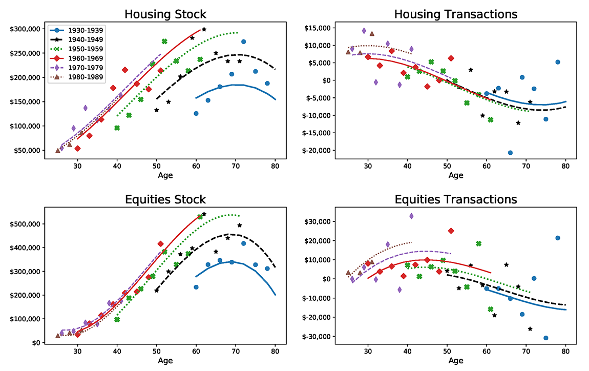
Note: Asset holdings and transactions, estimated in the Survey of Consumer Finances. Units are in constant January 2023 US dollars. Each dot corresponds to a particular cohort in a particular survey. Lines are polynomials in age and cohort. Source: SCF and author calculations.
Welfare and Wealth Gains and Losses
The top panel of figure 3 shows the change in our money metric welfare measure due to the change in the asset price path between the July 2021 CBO projection and the February 2023 CBO projection by age. The black line shows the overall welfare change (the sum of asset-specific welfare changes) while the colored lines show the contribution from each asset or liability class. The bottom panel of figure 3 shows the change in wealth for each age group.11
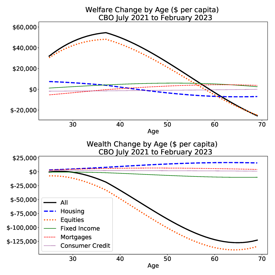
Note: Welfare and wealth changes by age. Units are constant January 2023 dollars. Source: CBO, SCF, and author calculations.
As the top panel shows, the asset price changes we consider had an inverted-u-shaped effect on welfare by age. The oldest individuals were hurt the most and would pay around $20,000 to revert to the July 2021 projection for asset prices. People around age 40 benefited the most and would have paid over $40,000 in July 2021 for the February 2023 asset price projection to come true. This lifecycle pattern is largely driven by the shape of the effects of equity prices, whose asset price changes have benefited the young, who are actively purchasing equities, at the expense of the old, who are selling equities.
A key takeaway from our analysis is that the change in wealth is not a good proxy for the change in welfare. The top panel in figure 3 shows that the age group that has benefited the most from the asset-price changes in this tightening cycle are those near age 40. By contrast, this age group has seen large declines in wealth.12
To understand the contrasting outcomes for welfare and wealth, consider the implications of the change in real equity prices, shown in the orange lines. Over the second half of 2021 and early 2022, equity prices dropped sharply, reflected in the steep wealth declines for older individuals. However, because the expected path for real interest rates has increased, the expected return on equities—which we project as a fixed spread above the short-term real rate—has increased. Furthermore, we assume the real dividends paid out from stocks are unchanged, so the income of an individual who holds the stock is unchanged. Individuals younger than sixty are, on net, buying equities they plan receive income from and then sell in retirement. Because they are buying equities cheaply and do not plan to immediately sell, they benefit from these changes in the stock market.
House prices, on the other hand, rose faster than expected between the July 2021 and February 2023 CBO projections, though the February projection falls below the July 2021 projection by 2025.13 The welfare and wealth effects of the house price surprise are shown in the blue lines. Higher house prices increased the wealth of older individuals who, on average, own more housing than younger individuals. In welfare terms, the updated path of house prices benefits young people who will likely buy houses in the coming years, when prices are predicted to be lower than the CBO had previously projected.14 The increase in mortgage rates hurts younger people the most, the effect of which is shown in the red lines. While young people must pay higher rates on the new mortgages they take out, older people have seen the real value of their existing mortgages decline with inflation, which directly increases their welfare.
Considerations
Our analysis leans on several assumptions and simplifications that we highlight in this section. One of the implications of our theory is that the welfare effects of asset price changes should add up to zero: for any buyer of an asset there is a seller for whom the asset price change will have an equal and opposite welfare effect. In practice, this is not the case for several reasons. First, much of the fixed income wealth is in the form of government debt, and we do not try to allocate the change in taxes, benefits, or government spending that will result from a change in the government's budget. Second, some assets are bought and sold by foreigners who do not appear in the SCF data. Third, the difficulty of imputing savings in each asset from SCF data mean that there is likely to be measurement error that does not net to zero.
We estimate the mean welfare change by age. This mean does not represent any one individual's experience, and given large differences in asset portfolios, individual welfare changes will vary widely around this mean. In particular, equity holdings are heavily skewed toward the top of the wealth distribution. Furthermore, we discount gains and losses at the same rate for all individuals. In reality, some people may be credit constrained and therefore place a higher value on gains that can be realized today versus at some time in the future relative to individuals who are not credit constrained.15 Furthermore, our measure is a first order approximation of welfare changes – although, as shown in Fagereng et al (2022), the second order effects are small. Relatedly, our analysis assumes perfect foresight over the future path of asset prices, and so we do not consider the welfare implications of changes in uncertainty.
To make our welfare model tractable, we have made simplifying assumptions about the mortgage market. We assume that people pay off their mortgage in full after 10 years and then refinance. This assumption overlooks the optionality embedded in most mortgage products: when mortgage rates go down individuals can refinance at the new, lower, rate. With mortgage rates having increased significantly from the July 2021 CBO projection, there is little value in this option for most existing mortgages.
Lastly, an essential aspect of this welfare calculation is that we only consider the effects of changes in asset prices. We ignore other changes in the economy, such as changes in the unemployment rate or fiscal policy. Therefore, our analysis speaks to the narrow question about the welfare implications of asset price changes only and does not seek to quantify recent welfare changes more generally. Moreover, other changes in the economy could lead to changes in asset purchasing behavior, and thereby change our welfare calculations. For example, rising unemployment among the middle-aged could lower their ability to purchase equities at lower prices and would reduce the welfare benefit of these lower prices.
Conclusion
The methodology in this note shows that over the period including the recent rise in inflation and subsequent monetary policy tightening, asset prices have moved in such a way as to, on average, benefit middle-aged people at the expense of retirees. While we think these results are useful to understand the heterogeneous effects of monetary policy, we note that the welfare effects we measure here are only those that arise from the redistribution of welfare through asset price changes. This measure does not capture the welfare effects of other large changes that have occurred in this period, such as in the labor market and in fiscal policy.
References
Andreas Fagereng, Matthieu Gomez, Emilien Gouin-Bonenfant, Martin Holm, Benjamin Moll, and Gisle Natvik (2022). Asset-price redistribution. Working paper.
Laura Feiveson and John Sabelhaus (2019). "Lifecycle patterns of saving and wealth accumulation," Finance and Economics Discussion Series 2019-010. Washington: Board of Governors of the Federal Reserve System, https://doi.org/10.17016/FEDS.2019.010r1.
1. The CBO does not explicitly forecast the 5-year treasury yield or an equity index. The projections shown for those asset prices are imputed by the authors. We provide more details about or methodology later in the note. Return to text
2. For our analysis, we sum from t=2021:Q3 to T=2041:Q4. T was chosen to be far enough in the future that price deviations at date T lead to small deviations in welfare. Return to text
3. We extend the methodology of Fagereng et al (2022) to address two considerations: (1) long-term debt and (2) the effects of inflation on the real value of nominal asset holdings. To calculate the welfare changes from longer term nominal debt, we first calculate the welfare change assuming the nominal interest rate has changed but that the inflation projection is unchanged. This is calculated as $$ \Delta Welfare_{a} \approx \sum_{t=0}^{T} R^{-t}((Sales_t-Debt Holdings_t )\times FractionMaturing+Sales_t)\times Price Deviation_t$$. Here the fraction of maturing debt is the reciprocal of the debt maturity. The price deviation is calculated by pricing a coupon bond before and after the interest rate change. We then calculate the change in welfare due to the change in the inflation projection as $$ \Delta Welfare_b \approx \sum_{t=0}^{T} R^{-t} Debt Holdings_{t} \times Inflation Deviation_{t} $$ The total welfare change is then the sum of $$ \Delta Welfare_a$$ and $$ \Delta Welfare_b$$. We set the annualized discount rate to be 5 percent following Fagereng et al (2022). Return to text
4. We assume fixed income assets and consumer credit liabilities have a maturity of 5 years and that defined contribution pensions, life insurance products, and other financial assets are composed of 50 percent equities and 50 percent fixed income assets. Return to text
5. We extend the results from Feiveson and Sabelhaus (2019) to include the 2019 wave of the SCF. We fit a polynomial (plotted in figure 2) in both age and cohort to the data and use constant extrapolation for cohorts younger than 1980-1989 and ages above 80. Return to text
6. Available at: https://www.cbo.gov/data/budget-economic-data. We extend the difference in the 10-year projections out to 20 years, assuming real price deviation closes in a linear fashion over the following 10 years. Our qualitative results are robust to other assumptions about the longer term, such as keeping the real price deviation fixed for the following 10 years. Return to text
7. The CBO releases new projections approximately every six months. February 2023 is the most recent projection. We chose the projection from July 2021 as the baseline because it is the last CBO forecast before the CBO expected interest rates to rise as fast as they have. Return to text
8. We assume a fixed equity premium of 4.5%. The equity premium is generally countercyclical and relative to July 2021, the most recent CBO projection has a somewhat higher projected unemployment rate, suggesting the equity premium may be higher than previously expected. However, our results are nearly identical if we assume the equity premium is higher over the next four quarters. Return to text
9. We also compute the liability holdings for mortgages and consumer credit over the lifecycle. Individuals take out mortgages and consumer credit at a high rate early in life and pay these debts down late in their working life and into retirement. Return to text
10. While millennials hold roughly the same amount of wealth in housing and equities as generation X did at the same age, the secular rise in the value of assets and the aging both mean that millennials hold a much smaller fraction of overall wealth than their parents did at the same age. Return to text
11. The change in wealth is the change in projected wealth of individuals in February 2023. Return to text
12. These findings contrast with the University of Michigan Survey of Consumer Expectations, which finds that middle-aged individuals report a large decline in the probability of a comfortable retirement. This difference could arise due to the salience of wealth losses, differences in expectations about future asset prices, or other factors that may have changed in the economy aside from asset prices. Return to text
13. In real terms, house prices fall below the July 2021 projection by the middle of 2023. Return to text
14. The welfare benefits of house price movements depend significantly on the dates we use. By July 2021, much of the rise in house prices had already happened or was forecast. If we had used an earlier date for comparison, young households would have been seen to have large welfare losses from the increase in house prices. Return to text
15. A further limitation of our welfare measure is that it does not account for the collateral value of higher asset prices for households that are credit constrained. Return to text
Crawley, Edmund, and William Gamber (2023). "Winners and losers from recent asset price changes," FEDS Notes. Washington: Board of Governors of the Federal Reserve System, May 12, 2023, https://doi.org/10.17016/2380-7172.3287.
Disclaimer: FEDS Notes are articles in which Board staff offer their own views and present analysis on a range of topics in economics and finance. These articles are shorter and less technically oriented than FEDS Working Papers and IFDP papers.