FEDS Notes
April 12, 2021
Inflation Thresholds and Policy-Rule Inertia: Some Simulation Results
Cristina Fuentes-Albero and John M. Roberts
In August 2020, the Federal Open Market Committee approved a revised Statement on Longer-Run Goals and Monetary Policy Strategy (FOMC, 2020) and in the subsequent FOMC meetings, the Committee made material changes to its forward guidance to bring it in line with the new framework. Clarida (2021) characterizes the new framework as comprising a number of key features. In this Note, we use simulations of the FRB/US model to assess possible consequences of several of them. First, the new framework introduces a new interpretation of the FOMC's maximum employment mandate. In the new framework, the FOMC will respond to "shortfalls of employment from its maximum level"—thus, the new framework is asymmetric. Second, the Committee expects to delay lift-off from the effective lower bound (ELB) until inflation reaches the target of 2 percent and it is likely to remain at or above that level on a sustained basis. Third, after lift-off, monetary policy is expected to remain accommodative for a while: The Committee "will likely aim to achieve inflation moderately above 2 for some time."
We conduct dynamic simulations using the public version of the FRB/US model and the public FRB/US database that builds on the December 2020 FOMC's Summary of Economic Projections under several monetary policy rules intended to capture features of the new framework. As explained in the Federal Reserve's semiannual Monetary Policy Report (FOMC, 2021), policymakers often consult prescriptions from simple interest rate rules as part of their monetary policy deliberations without mechanically following the prescriptions of any particular rule. While we examine rules that are intended to capture some features of the FOMC's new framework, they are only very rough approximations to the decision-making process the Committee is likely to adopt in practice. Moreover, the FRB/US model that we use to simulate the effects of various rules is just one model, and other models could—and likely would—have different predictions, even under the same rules.
Our starting point is the "balanced approach" rule discussed by Yellen (2017):
$$ (1) \ \ \ \ \ \ R_t = R^{\ast} + \pi_t + 0.5(\pi_t - \pi^{\ast}) + 1.0 * Y^{gap}_t, $$
where $$R_t$$ is the federal funds rate, $$R^{\ast}$$ is the level of the real federal funds rate that on average is expected to be consistent with the maximum employment and price stability mandates in the longer run, $$\pi_t$$ is current inflation, which we will measure with the four-quarter change in the index for core PCE prices, $$\pi^{\ast}$$ is the central bank's inflation objective, and $$Y_t^{gap}$$ is the output gap, defined as the percent deviation of real GDP from an estimate of its potential level.
We modify Equation 1 along the following lines to incorporate several of the new elements of the monetary policy framework. We introduce asymmetry by assuming that the coefficient on the output gap is zero when the gap is positive and one when the gap is negative. Therefore, the funds rate only reacts to shortfalls in economic activity. In addition, we incorporate a threshold criterion for the unemployment rate: The funds rate will remain at the ELB while the unemployment rate is above 4.1 percent.1 To reflect the intention to maintain the federal funds rate at its effective lower bound until inflation has risen to 2 percent, we supplement the rule with a threshold criterion related to inflation, which states that the federal funds rate will remain at the ELB until inflation has reached at least 2 percent. Finally, to reflect the idea that monetary policy will remain accommodative for some time after the funds rate has risen above its effective bound, we include inertia in the policy rule; including an inertial term ensures that the funds rate will rise only gradually toward the value consistent with the asymmetric balanced approach rule.
The following modified version of Equation 1 captures these features:
$$ (2) \ \ \ \ \ \ R_t = \begin{cases}\rho R_{t-1} + (1-\rho)[R^{\ast} + \pi_t + 0.5(\pi_t - \pi^{\ast}) + Y_t^{gap} \large{\mathbf{1}}\{Y_t^{gap} < 0\}] & , \pi_t > \pi_{thres}\ and\ u_t \le 4.1 \\ 0 & , \ otherwise \end{cases} $$
where $$\large{\mathbf{1}}\left\{Y_t^{gap}<0\right\}$$ is an indicator function that takes on a value of one when real GDP is below its potential level and zero when real GDP is higher than potential. To evaluate the ability of the enhanced rule to achieve inflation that is moderately above 2 percent for some time, we consider the effects of variation in two key parameters: two values for the inflation threshold ($$\pi_{thres}$$), 2 percent and 2.2 percent, and two values for the inertia parameter ($$\rho$$), 0.85 and 0.94.
We perform the model simulations using a baseline projection taken from the public FRB/US database that was posted in January 2021. As explained in Brayton, Laubach, and Reifschneider (2014), the public FRB/US databases is based on the median projection for the SEP variables where they are available. In our case, the public FRB/US database is based on the December 2020 SEP projection, which provided annual projections through 2023. The economy is then projected to converge gradually to the long-run values of the variables available in the SEP. We conduct our simulations of the alternative policies under the assumption that the economy is not subject to further shocks.
We use a version of the FRB/US model that assumes model-consistent expectations for financial market participants and for price and wage setters. Thus, these private-sector decisions are based on expectations that are fully informed about the structure of the economy and the conduct of monetary policy. As a result, these private-sector decision-makers understand the implications of each of the policy rules in real time. We assume that for other economic decisions, including the spending decisions of households and firms, expectations are not model consistent but are instead informed only by the historical co-movement between current data indicators and future variables as captured by vector autoregressions (VAR-expectations).2
We first assess the impact of the inflation threshold and policy inertia parameters under the asymmetric rule and then examine the corresponding results under a symmetric rule. Table 1 reports the date of lift-off from the ELB, the minimum value of unemployment reached during the simulation, the maximum value of inflation after 2021, and the average inflation level in the 2020-2030 period.3 Comparing the first two columns in Table 1, under the higher of the two inflation thresholds, the average inflation rate over the period of interest and the maximum value of inflation are both higher. As well, the additional accommodation translates into a lower minimum for the unemployment rate. The results are similar when assessing the effects of a higher inflation threshold in an economy characterized by a policy rule with higher inertia (the last two columns in Table 1).
Table 1: Results under asymmetric rules
| Low inertia | High inertia | |||
|---|---|---|---|---|
| Inflation threshold | 2% | 2.2% | 2% | 2.2% |
| ELB departure date | 2024Q2 | 2026Q3 | 2023Q2 | 2024Q1 |
| Minimum value of unemployment | 3.69 | 3.28 | 3.6 | 3.46 |
| Maximum value of inflation after 2021 | 2.02 | 2.23 | 2.17 | 2.22 |
| Average inflation 2020-2030 | 1.91 | 2.06 | 2.03 | 2.07 |
Note: Low inertia refers to an economy with a policy rule with a 0.85 inertia coefficient and high inertia stands for an economy with a policy rule with a 0.94 inertia coefficient.
We next assess the role played by inertia. Comparing the first and third columns in Table 1, which incorporate 0.85 and 0.94 inertia coefficients, respectively, assuming a 2 percent threshold criterion, lift-off is earlier with the higher inertia setting. Nonetheless, under higher inertia, unemployment reaches a slightly lower value while inflation is somewhat higher. With a 2.2 percent inflation threshold, differences in lift-off date are even more marked across different inertia coefficients. However, the inflation outcomes are very similar, and, in this case, the minimum unemployment rate is somewhat higher with greater inertia.
Figure 1 presents the simulated paths for several key variables under each of the policy rules. The upper right panel shows that under each of the options, there is some overshooting of the 2 percent inflation objective. The overshooting is substantial and long-lasting for rules with a 2.2 percent inflation threshold under either inertia coefficient. Under the lower inertia coefficient, there is only a very modest overshooting with a 2 percent inflation threshold. However, with the higher inertia coefficient, there is a significant and persistent overshooting of the target even with a 2 percent inflation threshold in the rule. As show by the upper left panel, under the 0.94 inertia coefficient, the paths for unemployment are quite similar for the two inflation thresholds. The thresholds have a bigger effect under an inertial term of 0.85, with the unemployment paths differing by as much as 65 basis points. The bottom panel illustrates that rules with higher inertia deliver more accommodative paths for the funds rate despite prescribing earlier liftoff dates.
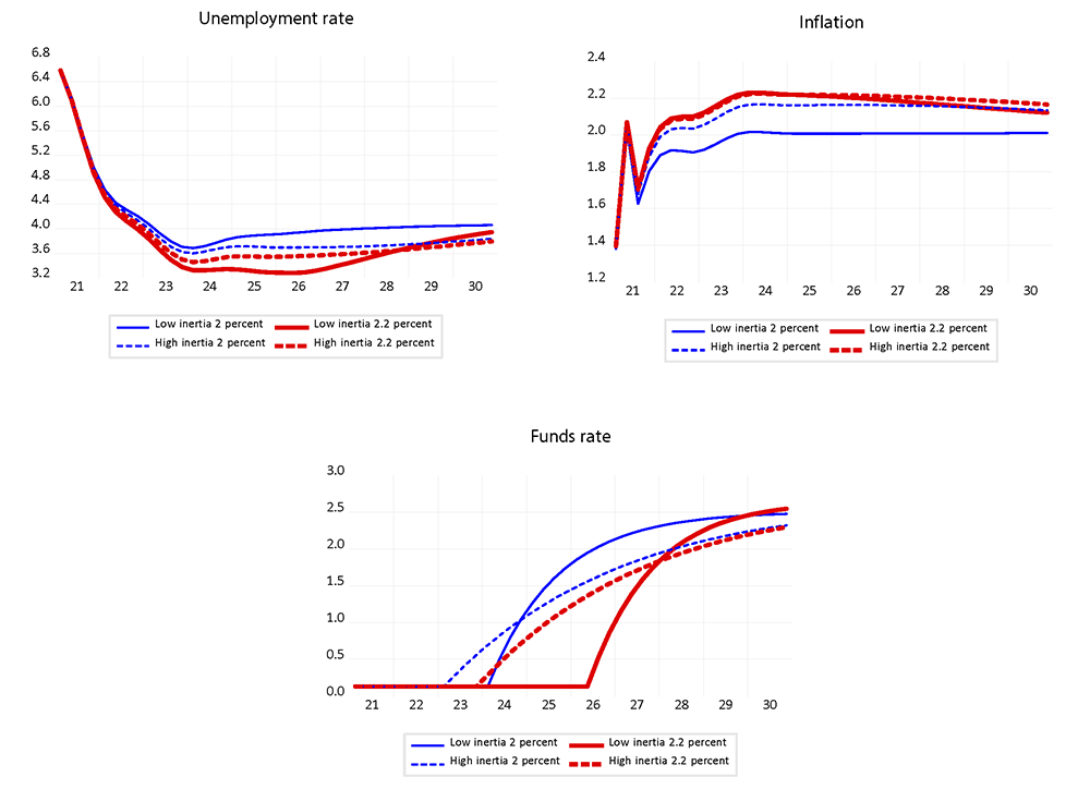
Note: Low inertia refers to an economy with a policy rule with a 0.85 inertia coefficient and high inertia stands for an economy with a policy rule with a 0.94 inertia coefficient.
In Table 2, we turn to the role of asymmetry in the rule, under the same inertial term and inflation threshold combinations as before but now assuming that the monetary authority responds to the output gap symmetrically. Thus, we assume as in Equation 1 that the monetary authority responds to both positive and negative output gaps with a coefficient of 1. Under the symmetric rules in Table 2, maximum inflation effects are slightly lower and liftoff from the ELB is delayed. In Figure 2, we report the simulated paths under a symmetric rule—circled solid line—and under an asymmetric rule—solid line—for the case with an inertia coefficient of 0.85 and an inflation threshold of 2.2. As shown in the upper panels, the simulated paths for unemployment and inflation are quite similar. However, the simulated path for the funds rate is steeper for a rule with a symmetric response to the output gap. The path for the funds rate is steeper because after liftoff, the output gap is positive and under a symmetric rule, the monetary authority responds to it by tightening. Under the asymmetric rule, the monetary authority does not respond to positive realizations of the gap by assumption, delivering a more accommodative path for the policy rate. Because inflation is slightly lower under the symmetric rule, lift-off from the effective lower bound is delayed. Conditional on our policy-rule specifications and the dataset used, our results point to little impact in terms of economic outcomes linked to the symmetry assumption in the policy rule. However, asymmetry could matter more in situations such as prolonged periods of positive output gaps and inflation around target.
Table 2: Results under symmetric rules
| Low inertia | High inertia | |||
|---|---|---|---|---|
| Inflation threshold | 2% | 2.2% | 2% | 2.2% |
| ELB departure date | 2024Q3 | 2027Q1 | 2023Q3 | 2025Q3 |
| Minimum value of unemployment | 3.68 | 3.29 | 3.64 | 3.37 |
| Maximum value of inflation after 2021 | 2.01 | 2.21 | 2.08 | 2.21 |
| Average inflation 2020-2030 | 1.9 | 2.04 | 1.96 | 2.05 |
Note: Low inertia refers to an economy with a policy rule with a 0.85 inertia coefficient and high inertia stands for an economy with a policy rule with a 0.94 inertia coefficient.
We summarize our results as follows:
- Under a 2 percent inflation threshold and a moderate degree of inertia in the policy rule (ρ=0.85), inflation only very modestly exceeds the FOMC's inflation objective.
- Either a slightly higher inflation threshold (2.2 percent) or a higher degree of policy-rule inertia (ρ=0.94) can lead to a modest overshooting of inflation, with inflation reaching 2.2 percent and averaging slightly higher than 2 percent over the decade ending 2030.
- We find in these simulations that the asymmetry of the reaction to the output gap in the policy rule has only a modest effect on outcomes for unemployment and inflation. However, this feature could matter more in other settings, such as under prolonged periods of positive output gaps.
Figure 2. Simulated paths under Taylor 99 with 2.2 percent inflation threshold: asymmetric vs symmetric rule
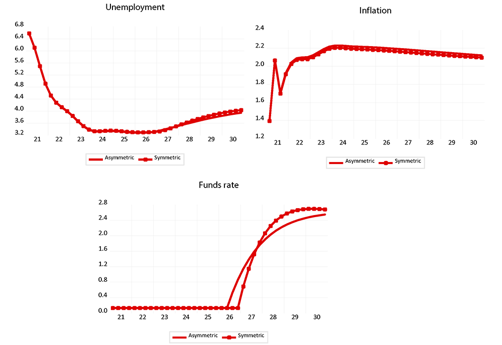
Note: Low inertia refers to an economy with a policy rule with a 0.85 inertia coefficient and high inertia stands for an economy with a policy rule with a 0.94 inertia coefficient.
References
Brayton, Flint, Thomas Laubach, and David Reifschneider (2014), "The FRB/US Model: A Tool for Macroeconomic Policy Analysis," FEDS Notes. Washington: Board of Governors of the Federal Reserve System, April 03, 2014.
Clarida, Richard H. (2021), "The Federal Reserve's New Framework: Context and Consequences," speech delivered at "The Road Ahead for Central Banks," a seminar sponsored by the Hoover Economic Policy Working Group, Hoover Institution, Stanford University, January 13 (via webcast).
Federal Open Market Committee (2020), "Statement on Longer-Run Goals and Monetary Policy Strategy".
Federal Open Market Committee (2021), Monetary Policy Report, February 19.
Yellen, Janet L. (2017), "The Economic Outlook and the Conduct of Monetary Policy," speech delivered at the Stanford Institute for Economic Policy Research, Stanford University, January 19.
1. The median of the Committee's projection for the rate of unemployment consistent in the longer run with 2 percent inflation was 4.1 percent in the December 2020 SEP. Return to text
2. The rule described in Equation 2 implies a "trigger" strategy under which the federal funds rate follows the rule as soon as the four-quarter change in core inflation exceeds 2 percent and the unemployment rate is below 4.1 percent. Under a pure trigger strategy, attaining the thresholds is necessary and sufficient for lift-off from the ELB. We found, however, that in some cases, such a pure trigger strategy cannot be realized in equilibrium. Because price- and wage-setters are forward-looking, the effects of forward guidance on inflation are front-loaded. Consequently, in some cases, there can exist an ELB duration such that the lift-off criterion is never met for an earlier ELB exit, while any later exit causes inflation to hit the trigger condition many quarters too soon. When the trigger strategy fails, we use a "minimal ELB length" criterion to date lift-off: Lift-off occurs at the date for which the ELB period is the shortest given that the thresholds for inflation and unemployment are met at some point before lift-off. Under this criterion, attaining the thresholds is necessary, but not sufficient, for lift-off. Return to text
3. These exercises are only illustrative. Thus, while the "lift-off" reported dates in Table 1 (and, later, in Table 2) are useful for comparing the impact of the different rules in the FRB/US model, they should not be read as providing a prediction of what the FOMC is likely to do in practice. Return to text
Fuentes-Albero, Cristina, and John M. Roberts (2021). "Inflation Thresholds and Policy-Rule Inertia: Some Simulation Results," FEDS Notes. Washington: Board of Governors of the Federal Reserve System, April 12, 2021, https://doi.org/10.17016/2380-7172.2899.
Disclaimer: FEDS Notes are articles in which Board staff offer their own views and present analysis on a range of topics in economics and finance. These articles are shorter and less technically oriented than FEDS Working Papers and IFDP papers.