Board of Governors of the Federal Reserve System

It is a pleasure and an honor to speak here today at the 60th Annual Meeting of the National Association for Business Economics (NABE). Since 1959, NABE has promoted the use of economics in the workplace and advanced the worthy purpose of ensuring that leading American businesses benefit from the insights of economists.

Today I will focus on the Federal Reserve's ongoing efforts to promote maximum employment and stable prices. I am pleased to say that, by these measures, the economy looks very good. The unemployment rate stands at 3.9 percent, near a 20-year low. Inflation is currently running near the Federal Open Market Committee's (FOMC) objective of 2 percent. While these two top-line statistics do not always present an accurate picture of overall economic conditions, a wide range of data on jobs and prices supports a positive view. In addition, many forecasters are predicting that these favorable conditions are likely to continue. For example, the medians of the most recent projections from FOMC participants and the Survey of Professional Forecasters, as well as the most recent Congressional Budget Office (CBO) forecast, all have the unemployment rate remaining below 4 percent through the end of 2020, with inflation staying very near 2 percent over the same period.¹

From the standpoint of our dual mandate, this is a remarkably positive outlook. Indeed, I was asked at last week's press conference whether these forecasts are too good to be true--a reasonable question! Since 1950, the U.S. economy has experienced periods of low, stable inflation and periods of very low unemployment, but never both for such an extended time as is seen in these forecasts.² Standard economic thinking has long offered an explanation for this: If unemployment were to remain this low for this long, employers would be pushing up wages as they compete for scarce workers, and rising labor costs would feed into more‑rapid price inflation faced by consumers.

This dynamic between unemployment and inflation is known as a Phillips curve relationship, and at times it can pose a fundamental tension between the two sides of the Fed's mandate to promote maximum employment and price stability. Recent low inflation and unemployment have some analysts asking, "Is the Phillips curve dead?"³ Others argue that the Phillips curve still lurks in the background and could reemerge at any time to exact revenge for low unemployment in the form of high inflation.

My comments today have two main objectives. The first is to explain how changes in the Phillips curve help account for the somewhat surprising but broadly shared current forecasts of continued very low unemployment with inflation near 2 percent. At the risk of spoiling the surprise, I do not see it as likely that the Phillips curve is dead, or that it will soon exact revenge. What is more likely, in my view, is that many factors, including better conduct of monetary policy over the past few decades, have greatly reduced, but not eliminated, the effects that tight labor markets have on inflation. However, no one fully understands the nature of these changes or the role they play in the current context. Common sense suggests we should beware when forecasts predict events seldom before observed in the economy.⁴

Thus, my second objective today is to explain, given this uncertainty about the unemployment-inflation relationship, the important role that risk management plays in setting monetary policy. I will explore the FOMC's monitoring and balancing of risks as well as our contingency planning for cases when risk becomes reality.

Historical Perspective on Jobs and Inflation
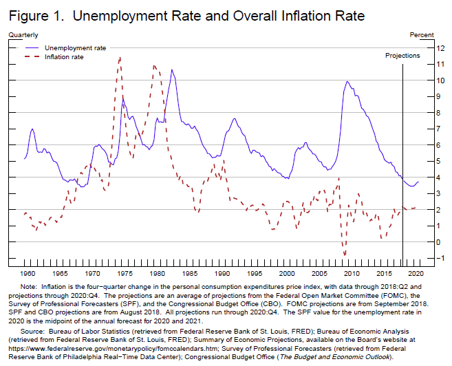
Let us start with a look at the modern history of jobs and inflation in the United States. Figure 1 shows headline inflation and unemployment from 1960 to today and extended through 2020 using the average of median projections from both FOMC participants and the Survey of Professional Forecasters, and the CBO projections. As the figure makes clear, a multiyear period with unemployment below 4 percent and stable inflation would, if realized, be unique in modern U.S. data.⁵

To understand the basis for these forecasts, it is useful to contrast two very different periods included in figure 1: From 1960 to 1985, and the period from 1995 to today. The first period includes the Great Inflation, and the latter includes both the Great Moderation and the distinctly immoderate period of the Global Financial Crisis and its aftermath.

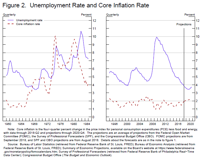
Figure 2 shows unemployment and core, rather than headline, inflation in these two periods. While our inflation objective concerns headline inflation, switching to core inflation makes some relationships clearer by removing a good deal of variability due to food and energy prices, variability that is not primarily driven by labor market conditions or monetary policy.

There is a dramatic difference in the unemployment-inflation relationship across these two periods. During the Great Inflation, unemployment fluctuated between roughly 4 percent and 10 percent, and inflation moved over a similar range. In the recent period, the unemployment rate also fluctuated between roughly 4 percent and 10 percent, but inflation has been relatively tame, averaging 1.7 percent and never declining below 1 percent or rising to 2.5 percent. Even during the financial crisis, core inflation barely budged. As a thought experiment, look at the right panel and imagine that you could see only the red line (inflation), and not the blue line (unemployment). Nothing in the red line hints at a major economic event, let alone the immense upheaval around the time of the global financial crisis.

Notice that, in each period, there is only one episode in which unemployment drops below 4 percent. In the late 1960s, unemployment remained at or below 4 percent for four years, and during that time inflation rose steadily from under 2 percent to almost 5 percent. By contrast, the late 1990s episode of below-4-percent unemployment was quite brief, and during the episode and surrounding quarters inflation was reasonably stable and remained below 2 percent.

To explore the Phillips curve relationship in these two periods more closely, we need to bring in the concept of the natural rate of unemployment. In standard economic thinking, an unemployment rate above the natural rate indicates slack in the labor market and tends to be associated with downward pressure on inflation; unemployment below the natural rate represents a tight labor market and is associated with upward inflation pressure.

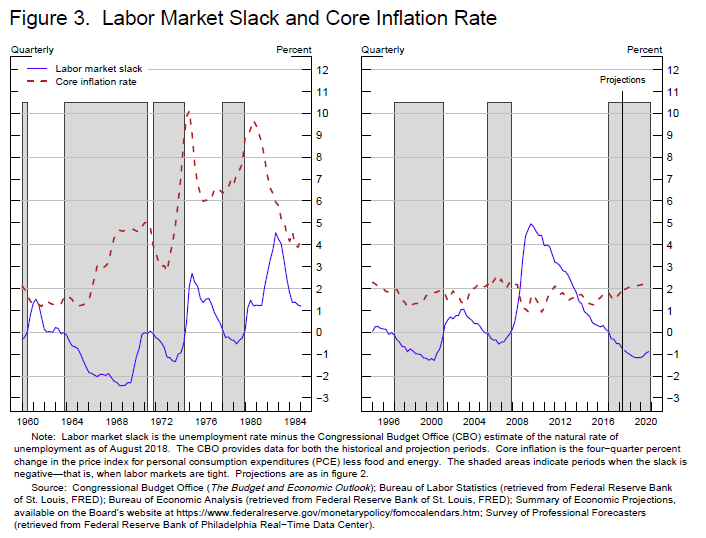
Figure 3 repeats figure 2 but replaces unemployment with labor market slack as measured by unemployment minus the CBO's current estimate of the natural rate of unemployment at each point in time.⁶ Periods of tight labor markets are shaded. During the Great Inflation, inflation generally rose in the tight, shaded periods and fell in the unshaded ones, just as conventional Phillips curve reasoning predicts.

From 1995 to today, the large and persistent swings in the gap between unemployment and the natural rate were associated with, at most, a move of a few tenths in the inflation rate. Comparing the shaded and unshaded regions, you might see some association between slack and the minor ups and downs in inflation, but the pattern is not at all consistent. It is evidence like this that fuels speculation about the Phillips curve's demise.

Whether dead, sick, or merely resting, many of the questions about the Phillips curve come down to figuring out what changed between these two periods, and why. Let us turn to a conceptual framework for examining these questions more systematically.

A Simple Framework for Understanding Changes in the Jobs-Inflation Relationship
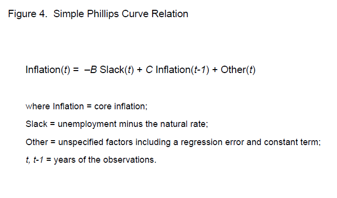
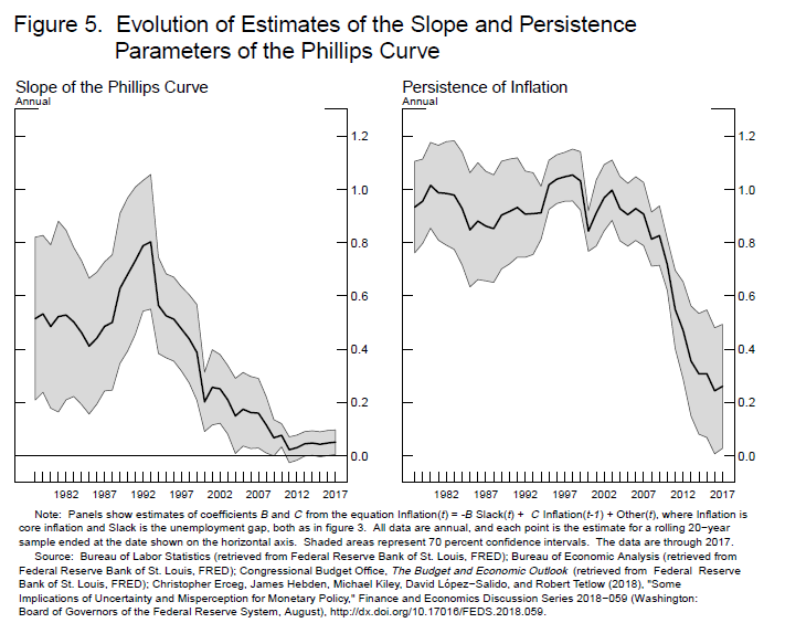
A natural starting point is the simplest form of a Phillips curve equation, which posits that inflation this year is determined by some combination of current labor market slack, inflation last year, and some other factors that I will leave aside for this discussion (figure 4):⁷

$$$$ Inflation(t)=-B Slack(t)+C Inflation(t-1)+Other(t)$$$$

The value of B is often referred to as the slope of the Phillips curve. With a larger value of B, any change in labor market slack translates into a bigger change in inflation. As we say, as B increases, the Phillips curve steepens. The value of C determines inflation's persistence--that is, how long any given change in inflation tends to linger. As the value of C increases, higher inflation this year translates more into higher inflation next year. A particularly nasty case arises when B and C are both large. In this case, slack has a large effect on inflation, and that effect tends to be very persistent. One implication of a large C is that, if a boom drives inflation up, it will tend to stay up unless offset by a subsequent bust.⁸

Figure 5 shows regression estimates of B and C, computed over 20-year samples starting with the sample from 1965 to 1984 and including each 20-year sample through 2017. During the Great Inflation samples, the value of C is near 1, meaning that higher inflation one year tended to translate almost one-for-one into higher inflation the next. The Phillips curve is also relatively steep in the Great Inflation samples, with 1 extra percentage point of lower unemployment converting into roughly 1/2 percentage point of higher inflation. Thus, the Great Inflation presented that nasty case just described.

Fortunately, things changed. The estimates of both B and C fall in value as the estimation sample shifts forward in time. In the most recent samples, the Phillips curve is nearly flat, with B very near zero, and C is about 0.25, meaning that roughly one fourth of any rise or fall in inflation carries forward. These results give numerical form to what we see in the right-hand panel of figure 3, covering the recent period: Large and persistent moves in the unemployment gap were associated with, at most, modest transitory moves in inflation.

What Led to the Changes in the Phillips curve?
These developments amount to a better world for households and businesses, which no longer experience or even fear the scourge of high and volatile inflation. To provide a sound basis for monetary policy, it is important to understand what happened and why, so we can avoid a return to the bad old days of the 1970s. Like many, I believe better monetary policy has played a central role.⁹

To understand the mechanism, let us ask how central banks could, presumably inadvertently, amplify and extend the duration of inflation's response to labor market tightness. To do so, the central bank could persistently ease the stance of monetary policy in response to an uptick in inflation. No responsible central banker today would intentionally do this, but much research suggests that during the Great Inflation, misunderstandings about how the economy worked led the Fed effectively to behave in this manner.¹⁰ Some policymakers may have believed the misguided notion that accommodating permanently higher inflation could purchase permanently higher employment.¹¹ Other policymakers misperceived the level of the natural rate of unemployment, which we now believe had shifted up markedly in the 1960s. With the higher natural rate, the labor market was much tighter and provided much greater upward pressure on inflation than policymakers realized in real time. As a result, they were continually "behind the curve."¹²

The channel through which monetary policy can amplify and extend inflation's response to shocks becomes even stronger when we take account of expectations. If people come to expect that upward blips in inflation will result in ongoing higher inflation, they will build that view into wage and price decisions. In this case, people's expectations become a force adding momentum to inflation, and breaking inflation's momentum can require convincing people to change their minds and behavior--never an easy task. Arguably, this is why a federal funds rate near 20 percent--roughly 10 percent in real terms‑‑was required in the early 1980s to turn the tide on high inflation. The cost, in the form of very high unemployment, is clear in the Great Inflation figures. The Great Inflation taught us that a main task of monetary policy is to keep inflation expectations anchored at some low level.

This idea is behind the adoption in recent decades of inflation targets, such as the Fed's 2 percent objective, by central banks around the world. When monetary policy tends to offset shocks to inflation, rather than amplifying and extending them, and when people come to expect this policy response, a surprise rise or fall in labor market tightness will naturally have smaller and less persistent effects on inflation. Research suggests that this reasoning can account for a good deal of the change in the Phillips curve relationship.¹³ It is also likely that many other factors have contributed to changes in inflation dynamics over recent decades. We do not fully understand the causes and implications of these changes, which raises risk management issues that I will take up now.¹⁴

A Favorable Outlook, but What Could Go Wrong?
To set the stage, let us return to the situation facing the FOMC. The baseline forecasts of most FOMC participants and a broad range of others show unemployment remaining below 4 percent for an extended period, with inflation steady near 2 percent. I have made the case that this forecast is not too good to be true and does not signal the death of the Phillips curve. Instead, the outlook is consistent with evidence of a very flat Phillips curve and inflation expectations anchored near 2 percent.

But we still must face the cautionary advice to beware when forecasts point to rarely seen outcomes. As a way of heeding this advice, the Committee takes a risk management approach, which has three important parts: monitoring risks; balancing risks, both upside and downside; and contingency planning for surprises. Let me describe a few of the risks and how we are thinking about them.

Could Inflation Expectations Become Unanchored?
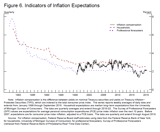
First is the risk that inflation expectations might lose their anchor. We attribute a great deal of the stability of inflation in recent years to the anchoring of longer-term inflation expectations. And we are aware that it could be very costly if those expectations were to drift materially. As you probably know from our public communications, we carefully monitor survey- and market-based proxies for expectations, and we do not see evidence of a material shift in longer-term expectations (figure 6). The survey measures have been particularly steady for some time.¹⁵ The financial market-based measures include both an expectations component and a volatile inflation premium component, so they tend to move around much more than the surveys, but we see no evidence of a material change in these measures, either.

The risks to inflation expectations are, of course, two sided. Until this summer, inflation had remained stubbornly below 2 percent for several years. And major economies in much of the world have been struggling mainly with disinflationary forces. Thus, we have been and will remain alert for possible downward drift in expectations. Some argue the contrary case--that by only gradually removing accommodation as the unemployment rate has fallen, the FOMC may have fallen behind the curve, thereby risking an upward drift in expectations. From the standpoint of contingency planning, our course is clear: Resolutely conduct policy consistent with the FOMC's symmetric 2 percent inflation objective, and stand ready to act with authority if expectations drift materially up or down.

Could Inflation Pressures Move up More than Expected in a Hot Economy?
A second risk is that labor market tightness or tightness in other parts of the production chain might lead to higher inflation pressure than expected--the "revenge of the Phillips curve" scenario.¹⁶ As I mentioned, the FOMC carefully monitors a wide array of early indicators of inflation pressure to evaluate this risk. Wages and compensation data are one important source of information. These measures have picked up some recently, but in a way that is quite welcome. Specifically, the rise in wages is broadly consistent with observed rates of price inflation and labor productivity growth and therefore does not point to an overheating labor market. Further, higher wage growth alone need not be inflationary. The late 1990s episode of low unemployment saw wages rise faster than inflation plus productivity growth without an appreciable rise in inflation.

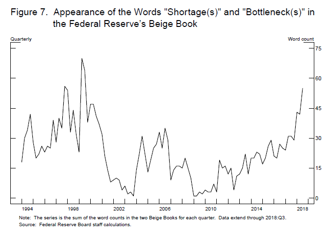
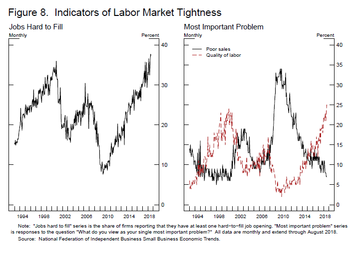
Despite what shows up in the aggregate wage and compensation data, however, I am sure that, like us, many of you are hearing widespread anecdotes about labor shortages and increasing bottlenecks in production. For example, as shown in figure 7, the words "shortage" and "bottleneck" are increasingly appearing in the Beige Book, the Federal Reserve's report summarizing discussions with our business contacts around the country.¹⁷ The message we are hearing in our conversations is supported by a wide range of more conventional measures. For example, the survey of members of the National Federation of Independent Business finds firms increasingly reporting that job openings are hard to fill (figure 8). Further, these businesses now list "quality of labor" as their most important problem, as opposed to the more typical report of "poor sales."

We review a wide variety of measures of this type, and these indicators show what I think most business people see: an economy operating with limited slack. Notice, however, that these measures are near levels that prevailed in the late 1990s or early 2000s, a period when core inflation remained under 2 percent.

While the late 1990s case proves that elevated values of these tightness measures do not automatically translate into rising inflation, a single episode provides only limited reassurance. Thus, the FOMC takes seriously the possibility that tight markets for labor or other inputs could provide greater upward pressure on inflation than in the baseline outlook. Our best estimates, however, suggest that so long as inflation expectations remain anchored, a modest steepening of the Phillips curve would be unlikely to cause a significant rise in inflation or demand a disruptive policy tightening.¹⁸ Once again, the key is the anchored expectations.

Is the Natural Rate of Unemployment Lower Than Expected?
A third risk--in this case an upside risk--is that the natural rate of unemployment could be even lower than current estimates. Some have argued that the Fed should be removing policy accommodation much more slowly, pushing the economy to see if the natural rate of unemployment is lower still.

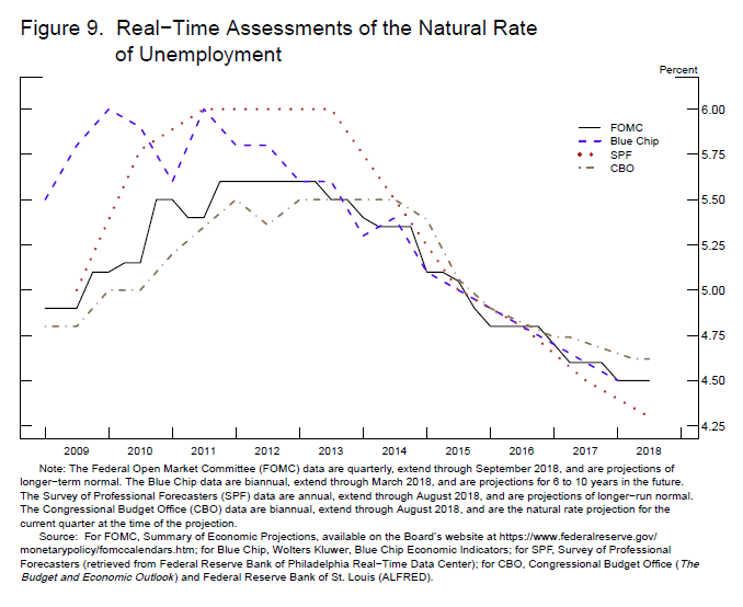
Advocates of this view note that over the past several years of policy normalization, the economy has continued to strengthen and unemployment has fallen, but inflation has remained quiet. As I discussed in a recent speech, many analysts have accounted for the lack of rising inflation pressure by lowering their estimate of the natural rate.¹⁹ For example, since the start of 2016, the unemployment rate has fallen about 1 percentage point, and estimates of the natural rate from four well-known sources have fallen over that period between 0.3 percent and 0.7 percent (figure 9).

If the natural rate is now materially lower than we believe, that would imply less upward pressure on inflation--the flip side of the "revenge of the Phillips curve" risk. Our policy of gradual interest rate normalization represents the FOMC's attempt to take both of these risks seriously. Removing accommodation too quickly could needlessly foreshorten the expansion. Moving too slowly could risk rising inflation and inflation expectations. Our path of gradually removing accommodation, while closely monitoring the economy, is designed to balance these risks.

In wrapping up this discussion of risks to the favorable outlook, I should emphasize that I have chosen to focus on three risks that are all associated with the Phillips curve. There are, of course, myriad other risks. To name just a few, we must consider the strength of economies abroad, the effects of ongoing trade disputes, and financial stability issues. I hope my discussion of three particular risks gives a sense of how we approach these issues.

Conclusion
Many of us have been looking back recently on the decade that has passed since the depths of the financial crisis. In light of that experience, I am glad to be able to stand here and say that the economy is strong, unemployment is near 50-year lows, and inflation is roughly at our 2 percent objective. The baseline outlook of forecasters inside and outside the Fed is for more of the same.

This historically rare pairing of steady, low inflation and very low unemployment is testament to the fact that we remain in extraordinary times. Our ongoing policy of gradual interest rate normalization reflects our efforts to balance the inevitable risks that come with extraordinary times, so as to extend the current expansion, while maintaining maximum employment and low and stable inflation.

References
Bernanke, Ben S. (2007). "Inflation Expectations and Inflation Forecasting," speech delivered at the Monetary Economics Workshop of the National Bureau of Economic Research Summer Institute, Cambridge, Mass., July 10.

Blanchard, Olivier (2016). "The U.S. Phillips Curve: Back to the 60s? (PDF)" Policy Brief PB16‑1. Washington: Peterson Institute for International Economics, January.

Blinder, Alan S. (2018). "Is the Phillips Curve Dead? And Other Questions for the Fed," Wall Street Journal, May 3.

Erceg, Christopher, James Hebden, Michael Kiley, David López-Salido, and Robert Tetlow (2018). "Some Implications of Uncertainty and Misperception for Monetary Policy," Finance and Economics Discussion Series 2018-059. Washington: Board of Governors of the Federal Reserve System, August.

Gordon, Robert J. (2018). "Friedman and Phelps on the Phillips Curve Viewed from a Half Century's Perspective," NBER Working Paper Series 24891. Cambridge, Mass.: National Bureau of Economic Research, August.

Kiley, Michael T. (2015). "Low Inflation in the United States: A Summary of Recent Research," FEDS Notes. Washington: Board of Governors of the Federal Reserve System, November 23.

Pfajfar, Damjan, and John M. Roberts (2018). "The Role of Expectations in Changed Inflation Dynamics (PDF)," Finance and Economics Discussion Series 2018-062. Washington: Board of Governors of the Federal Reserve System, August.

Powell, Jerome H. (2018). "Monetary Policy in a Changing Economy," speech delivered at "Changing Market Structure and Implications for Monetary Policy," a symposium sponsored by the Federal Reserve Bank of Kansas City, held in Jackson Hole, Wyo., August 23-25.

Romer, Christina D., and David H. Romer (2002). "The Evolution of Economic Understanding and Postwar Stabilization Policy (PDF)," paper presented at "Rethinking Stabilization Policy," a symposium sponsored by the Federal Reserve Bank of Kansas City, held in Jackson Hole, Wyo., August 29-31.

Stein, Herbert (1998). What I Think: Essays on Economics, Politics, and Life. Washington: AEI Press.

Yellen, Janet L. (2015). "Inflation Dynamics and Monetary Policy," speech delivered at the Philip Gamble Memorial Lecture, University of Massachusetts, Amherst, September 24.

-------- (2017). "Inflation, Uncertainty, and Monetary Policy," speech delivered at "Prospects for Growth: Reassessing the Fundamentals," 59th Annual Meeting of the National Association for Business Economics, Cleveland, Ohio, September 26.

---

1. I am referring to the most recent forecast for year-end 2018 through 2020. The unemployment rate for each forecast bottoms out at 3.4 percent or 3.5 percent in 2019 and remains below 4 percent. Headline PCE (personal consumption expenditures) inflation is between 1.9 percent and 2.1 percent for all three years and forecasts. The sources for the forecast data are given in the notes to figure 1. Return to text

2. For example, there have been four periods with quarterly average unemployment below 4 percent since 1950. In an early 1950s episode, inflation ranged from below zero to 8 percent. Toward the end of the 1950s, unemployment was near 4 percent for a time, dipping to 3.9 percent for one quarter. During this low unemployment period, inflation rose steadily from under 1 percent to over 3 percent. The remaining two episodes with unemployment under 4 percent--one each in the 1960s and 1990s--are discussed later in the speech. Return to text

3. This question is asked in the title of a recent editorial by Alan Blinder (2018), and a Google search reveals many similar titles. The research on the topic is reviewed more fully later in the speech. Return to text

4. Herb Stein (1998) made the analogous point that one should doubt the assertion that some program will "cause the economy to perform outside the range of its past experience" (p. 217). Return to text

5. See note 2. Unless otherwise noted, all statements about inflation will be four-quarter percent changes in quarterly average data, and all statements about unemployment will be about the quarterly average unemployment rate. Return to text

6. This estimate is the CBO's current assessment of what the natural rate was at each period in the sample, not a measure of the natural rate as perceived in real time. I discuss the importance of this distinction in Powell (2018). Return to text

7. What is reported here is an updated version of results reported in Erceg and others (2018), and that work provides additional discussion. Note that the "Other" term includes a constant. Return to text

8. The text refers to when C is less than 1, in which case a rise in inflation would ultimately die out on its own. When C is 1, the Phillips curve is of the "accelerationist" variety, and any offsetting rise in inflation due to labor market tightness would be permanent unless offset by an equal amount of subsequent slack. Blanchard (2016) has a good discussion of this issue. Return to text

9. The account I present of the role of anchored expectations in stabilizing the economy and favorably altering Phillips curve dynamics echoes a long-held view at the Fed. See Bernanke (2007) and Yellen (2015). Kiley (2015) reviews the recent research literature on this topic. Blanchard (2016) presents a very similar perspective. Return to text

10. To be clear, during the periods of rising inflation in the 1960s and 1970s, the FOMC was generally raising the federal funds rate, but with inflation rising, the real federal funds rate was rising much more slowly or even falling. In this sense, the effective stance of policy was tightening slowly or was easing. Return to text

11. Romer and Romer (2002) make this argument. Return to text

12. I discuss this argument in greater depth in Powell (2018). Return to text

13. Yellen (2017) gives a more detailed account of how a very flat Phillips curve with anchored expectations can account well for the recent inflation and unemployment data. See also note 9. Return to text

14. Many changes not directly related to policy might nonetheless have been precipitated by the improvement in policy. For example, Pfajfar and Roberts, (2018) present evidence that when inflation is more stable, people simply pay less attention to it and that this could help account for changes in the Phillips curve relationship. Return to text

15. That is, movements in these measures have been modest, especially taking into account precision of the surveys. Return to text

16. Gordon (2018) presents one version of the revenge hypothesis. Return to text

17. The length of the Beige Book has varied somewhat over time; for example, the Beige Book was redesigned in 2017, with the number of words reduced about 10 percent. It is unclear whether the number of important words like "shortage" would have been affected by that redesign, but if so, it would go in the direction of holding down the observed recent increase. Return to text

18. See, for example, Erceg and others (2018). Return to text

19. See Powell (2018). Return to text