Three-Factor Nominal Term Structure Model
This is a no-arbitrage dynamic term structure model, implemented as in Kim and Wright1 using the methodology of Kim and Orphanides2. The underlying model is the standard affine Gaussian model with three factors that are “latent” (i.e., the factors are defined only statistically and do not have a specific economic meaning). The model is parameterized in a maximally flexible way (i.e., it is the most general model of its kind with three factors that are econometrically identified). In the estimation of the parameters of the model, data on survey forecasts of 3-month Treasury bill (T-bill) rate are used in addition to yields data in order to help address the small sample problems that often pervade econometric estimation with persistent time series like bond yields.
A dynamic term structure model, like the one implemented here, can be used to extract market expectations of the future path of the short rate, term premiums in bond yields, etc. Of course, if the so-called expectations hypothesis were to hold, the instantaneous forward rate curve (or, more accurately, the futures rate curve) would equal the expected path of the short rate, the term premium would be zero, and there would be no need for complicated modeling to read off market expectations about the path of the short rate. While market participants have often used forward/futures rate as the expected future short rate, especially for relatively short horizons, many observers doubt that longer-horizon forward rates, which fluctuate a lot, adequately represent the movements of long-horizon expectations. Indeed, a large body of empirical literature has documented the failure of the expectations hypothesis. Dynamic term structure models operationalize the idea that bond yields embed premiums for interest rate risk (which could be positive or negative), and can be viewed as modeling the departures from the expectations hypothesis while still maintaining certain sensible assumptions about the behaviors of yields and term premiums (e.g., that these are smooth functions of time-to-maturity).
Q&A
- How are term premiums defined?
Here, term premiums are defined as departures from the expectations hypothesis. Thus, the term premium in yields is defined as yield minus the expected average short rate (over the life of the bond), and the term premium in forward rates is defined as forward rate minus the expected short rate (for the same horizon as the forward rate contract). This way of defining term premium embeds the so-called convexity premium in the term premium. In other words, our definition of term premium can be written as “term premium = pure term premium + convexity premium”. The “pure term premium” reflects compensation for interest rate risk. The convexity premium arises from the nonlinearity in the relationship between bond prices and yields; if the expected path of short rates was flat and the pure term premium was zero, the yield curve should have a slightly negative slope because the convexity premium contributions are negative. An alternative definition of term premium used in the literature3 corresponds to what we refer to as the “pure term premium” here, i.e., a measure that excludes the convexity premium. Because the magnitudes of convexity premiums tend to be fairly small, the difference between the two term premium definitions is often negligible; this is especially the case when looking at the changes in term premiums. However, when comparing the levels of term premiums, it may be worthwhile to keep in mind that our “term premium” is mechanically slightly lower than the “pure term premium” because of the negative convexity premium. - Is there something special about having three factors?
No. The model can be in principle implemented for any number of factors. Some practical considerations do constrain the number of factors that are typically used: too few factors could render the model too limited in describing the rich behavior of the yield curve, while too many factors could raise tractability issues and overfitting concerns. The latter denotes the problem that, even if one succeeds in estimating a model with large number of parameters, the estimated model could be fragile and could have unreliable implications for those aspects of the model that were not explicitly fitted. For example, if the model has a large number of factors, it can fit observed bond yields very closely, since the model implementation explicitly tries to minimize those fitting errors. However, it doesn’t guarantee that objects that are not explicitly fitted, such as multi-period expectations and term premiums, have more sensible properties than in a model with smaller number of factors.
Following many other works in this area, the present implementation of the model uses three factors. With three factors, the fitting error for yields could still be sizeable at times. For example, as of August 2019, the model-implied 10-year yield was about 10 basis points higher than observed yield, and the model-implied 5-year yield was about 5 basis points lower than observed yield. - Why are survey forecast data used in the estimation of the model in addition to yields data?
Standard estimation of flexibly specified dynamic term structure models (with yields data alone) can often produce results that have questionable implications for the expected path of the short rate and term premiums. Of course, objects like expected future interest rates and term premiums are not directly observable. However, most observers can agree that certain behaviors of interest rate expectations would be clearly unreasonable. For example, relatively long-horizon expectations of the nominal short rate, say the expectation of the short rate over the next 5 to 10 years, is believed to have come down significantly since the 1980s, as longer-horizon inflation expectations declined over time and got better anchored around the FOMC’s stated objective of 2 percent inflation target(PCE inflation). But a number of dynamic term structure models implemented in a standard way have often produced model-implied 5-to-10-year expected short rate that has changed little over a sample period that goes back to the 1980s or 1990s. Such a model would automatically attribute almost all of the variation in 5-to-10-year forward rate to the variation in the term premium component of the forward rate, and therefore miss a meaningful variation in the expectations component.4 For another example, when the Federal Reserve began raising the target funds rate in June 2004, the market is believed to have quickly coalesced on interpreting the FOMC’s “measured” pace language as one quarter-point hike per meeting, thus on a near-term expected pace of about 2 percent per year. But a number of standard implementations of dynamic term structure models showed (and still show) a notably shallower path of the short rate than that, hence quite sizeable (and positive) term premiums, for the second half of 2004.5 Furthermore, standard estimations tend to generate very wide confidence intervals for objects of interest such as term premiums (i.e., the estimates of key objects are very imprecise).
Econometrically, these problems are known as the “small sample problem.”6 Bond yields are fairly persistent time series. Therefore in order to reliably estimate the parameters of a flexibly specified term structure model, one needs a sample that spans a long period; sampling a given period more frequently (e.g., changing the sampling frequency to daily frequency) will not help solve the problem. Researchers have considered several approaches to addressing this problem. One is to use a longer sample period. However, using a somewhat longer sample (say, 10 more years of data) does not necessarily guarantee that the problem will go away; furthermore, extending the sample further back into the past can raise questions about the structural stability of the model. For example, some researchers have argued that the period before the Volcker disinflation could have had different interest rate dynamics than the period after, and shocks were generally larger before the Great Moderation period (1980s and 90s); therefore including the period before that could overstate the model-implied uncertainty about the future path of interest rates.
Another approach to address the small sample problem is to add restrictions on the term structure model to impose more discipline. As an extreme example, if all of the model parameters that determine the so-called market price of risks are set to zero (this amounts to saying that there is no compensation for bearing interest rate risk), the model effectively becomes identical to the so-called expectations hypothesis. But such a restriction would likely be viewed as too drastic, given the extensive evidence against the expectations hypothesis. While it might be possible to impose restrictions on the model in a less drastic way, a well-accepted set of restrictions has not emerged in the literature. Current implementation therefore uses survey data on the forecast of the three-month T-bill yield in the estimation of the model (in addition to yields data) to provide more information that helps pin down the parameters that were hard to pin down reliably in the yields-only estimation. This does not mean that the survey forecasts are taken at face value; rather, the implementation assumes that the survey forecasts are a noisy proxy for the true expectations.7 - Are the data currently available at this website the same as what used to be available at the website for the FEDS working paper 2005-33? If not, what are the differences?
No. The data that used to be available at the web page for the FEDS working paper 2005-33 was based on an implementation using the parameters estimated before the Financial Crisis, while the data currently available on this site are based on an implementation using a more recent parameter estimate.
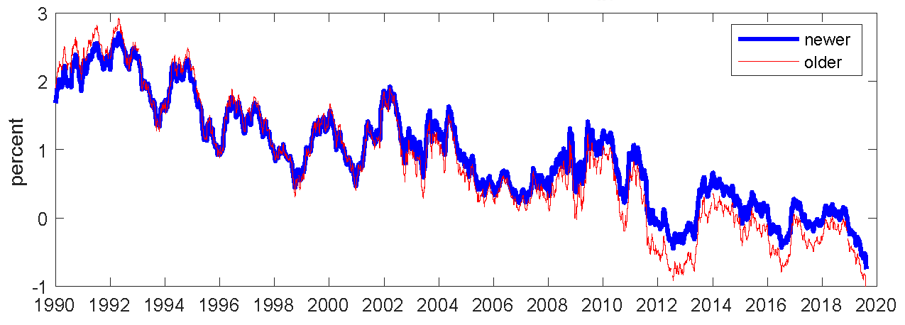
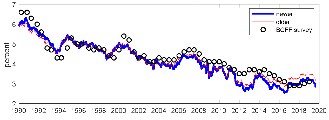
In principle, the model does not require a frequent re-estimation of the model’s parameters; in fact, it is the underlying assumption of the model that its parameters are stable (i.e., does not change over time).8 Furthermore, as discussed in question 3, adding several more years of yields data to the estimation sample by itself generally does not help resolve the aforementioned small sample problem. However, the implementation based on the old parameter estimate did lead to some undesirable features in the post-Financial-Crisis years ( e.g., the model-implied expected path of the short rate showed relatively fast mean-reversion even during the years when the short rate was stuck at the effective lower bound (ELB) and there was strong forward guidance, making the near-term term premiums more negative than can be considered reasonable.). It appeared that the ELB years that followed the Financial Crisis, or at least some aspects of them, were difficult to capture well with the previous parameter estimate. Therefore, the model was re-estimated with data that include the ELB years, and it is those data that are provided here. These (newer) data indeed have the feature that the near-term term premiums during the ELB years are not as negative as in the previous data. In the case of the 10-year yield term premium, as can be seen in the top panel of the chart below, the newer estimate and the older estimate have similar qualitative behaviors, though the level of the 10-year yield term premium from the older estimate has been modestly lower than that of the newer estimate in recent years. The bottom panel shows the time series of the model-implied 5-to-10-year expected average short rate based on the newer and older estimates. While both series are roughly consistent with the “long horizon” consensus forecast of the three-month T-bill yield from the Blue Chip Financial Forecasts (BCFF) survey, the newer estimate has a somewhat lower level in recent years relative to the older estimate.
It should be noted that the affine Gaussian model implemented here has limitations in capturing the dynamics of yields during the ELB years, and these limitations are shared by all models of this class, regardless of how many factors they have. For example, because the short rate has been practically stuck at the lower bound during the ELB years, estimated shocks from the affine Gaussian model are correlated during the ELB years,9 though the model assumes that those shocks are independent. The estimates presented here can be viewed as an attempt to parse the information in the current and past yield curves through the prism of a relatively tractable dynamic term structure model. It is important, however, to keep in mind that term structure models are not panaceas, that the expectations and risk attitudes which determine bond yields in the market may be exceedingly complex, that models are only approximate representations of the rich behaviors of the yield curve and the economy, and that caution is always warranted in interpreting outputs from models.
- How often do you re-estimate the parameters of the model?
The parameters of the model are not often re-estimated. (See the discussion in question 4.) With each new day’s yields data, the latent factor estimates are updated, which are then used to compute various model-implied properties such as expected future short rate and term premiums.
- How often are the data updated?
We generally try to post the updated series once per week; typically, updated series data will be posted on Tuesday for the period up to the Friday of the previous week. - Is this model an official Board statistical release?
No, this model is a staff research product and not an official statistical release. Accordingly, it is subject to delay, revision, or methodological changes without advance notice.
Model disclaimer
1. See Don H. Kim and Jonathan H. Wright, "An Arbitrage-Free Three-Factor Term Structure Model and the Recent Behavior of Long-Term Yields and Distant-Horizon Forward Rates" (Washington: Board of Governors of the Federal Reserve System, 2005). Return to text
2. See Don H. Kim and Athanasios Orphanides, “Term Structure Estimation with Survey Data on Interest Rate Forecasts,” Journal of Financial and Quantitative Analysis, 47 (February 2012): 241-272. Return to text
3. See, for example, Tobias Adrian, Richard K. Crump, and Emanuel Moench, “Pricing the Term Structure with Linear Regressions,” Journal of Financial Economics, 110 (October 2013): 110-138. Return to text
4. Note that a mismeasurement of the 5-to-10-year expected short rate will have an adverse effect on the measurements of objects like the 10-year yield term premium: if the 5-to-10-year expected short rate is over-estimated (under-estimated), the 10-year yield term premium will tend to be under-estimated (over-estimated). Return to text
5. Kim and Orphanides (2012, Figure 1) gives a related example in which a standard estimation of the dynamic term structure model using only bond yields data produced an implied path of the expected short rate at the end of 2013 that was too shallow to be plausible, given the macroeconomic backdrop at the time. Return to text
6. For more discussions of the small sample problem, see Kim and Orphanides (2012) and Canlin Li, Andrew Meldrum, and Marius Rodriguez (2017), "Robustness of long-maturity term premium estimates", FEDS Notes. Washington: Board of Governors of the Federal Reserve System, April 3, 2017. Return to text
7. As noted in Kim and Orphanides (2012), one can either let the model (and data) determine how noisy the survey data are, or impose a priori a specific amount of confidence about the survey data. Return to text
8. One might intuitively think that the likely change in market participant’s perception of the “neutral” rate over time would be more consistent with time-variation in some parameters. But that kind of effect is captured in the present model (though likely imperfectly) with time-variation in latent factors. Return to text
9. Because the short rate in the model is a linear combination of the factors, and because the short rate practically did not move during the ELB years, a linear combination of shocks during that period have to add up to zero, implying that they cannot all be independent. Return to text