FEDS Notes
June 30, 2023
A New Index to Measure U.S. Financial Conditions
Andrea Ajello, Michele Cavallo, Giovanni Favara, William B. Peterman, John W. Schindler IV, and Nitish R. Sinha1
(Updated: June 22, 2026)
FCI-G Data (baseline): Monthly (CSV) | Quarterly (CSV) | Data Definitions (PDF)
FCI-G Data (one-year lookback): Monthly (CSV) | Quarterly (CSV) | Data Definitions (PDF)
FCI-G Code (ZIP)
Note: On March 28, 2024, the quarterly data were updated to exclude a value for the month of February 2024, which is not a quarter-end month.
Starting with the January 2024 release, we will provide updated estimates underlying both Figure 1 and Figure 3 in this note, and share the code used to compute these estimates.
This note proposes a new index that can be used to gauge broad financial conditions and assess how these conditions are related to future economic growth.2 The index is broadly consistent with how the FRB/US model generally relates key financial variables to economic activity.
"Financial conditions" is a somewhat vague economic concept but typically refers to a constellation of asset prices and interest rates that are influenced by a variety of factors—including monetary policy—and have the potential to affect the real economy. Because of the ambiguous definition, measuring financial conditions is challenging. The common approach is to summarize the information content of a broad range of financial variables with a single indicator, commonly known as a financial conditions index (FCI).
Existing FCIs differ in the way they summarize financial market conditions both in terms of variables considered and the methodology used to extract the information content of these variables. Some FCIs use principal components or dynamic factor analysis to estimate common unobservable drivers of a broad set of financial variables (for example, the Federal Reserve Bank of Chicago's National Financial Conditions Index or the Bloomberg FCI). The main drawback of such an approach is that the weights used to aggregate the underlying financial variables are based on statistical models and do not necessarily have a straightforward economic interpretation, nor do they map changes in financial variables directly into measures of economic activity. Other FCIs weigh financial variables based on their contribution to expected economic activity as implied by stylized macroeconomic models (for example, the Goldman Sachs FCI) but typically do not take into account the lagged effects of financial variables.
In the spirit of model-based FCIs, the index introduced in this note aggregates changes in seven financial variables—the federal funds rate, the 10-year Treasury yield, the 30-year fixed mortgage rate, the triple-B corporate bond yield, the Dow Jones total stock market index, the Zillow house price index, and the nominal broad dollar index—using weights implied by the FRB/US model and other models in use at the Federal Reserve Board. These models relate households' spending and businesses' investment decisions to changes in short- and long-term interest rates, house and equity prices, and the exchange value of the dollar, among other factors.3 These financial variables are weighted using impulse response coefficients (dynamic multipliers) that quantify the cumulative effects of unanticipated permanent changes in each financial variable on real gross domestic product (GDP) growth over the subsequent year. The resulting index is named Financial Conditions Impulse on Growth (FCI-G).
While existing FCIs typically measure whether financial conditions are tight or loose relative to their historical distributions, the new index assesses the extent to which financial conditions pose headwinds or tailwinds to economic activity. Another important difference of this new index, compared with other commonly used FCIs, is its explicit consideration of the lags through which changes in financial variables are estimated to affect future economic activity. In the models used to construct the FCI-G, past changes typically receive decreasing weights, reflecting the diminishing effects that changes in financial variables have on economic activity over time.
As changes in financial variables work their way through the economy with lags, we use a lookback window—the length of the period over which past changes in financial variables are included in the calculation of the index—of either one or three years. Depending on the lookback window, more distant changes in financial variables drop out from the computation of the index after either one or three years.4 The step-by-step derivation of the index, along with the set of weights used for its construction, is provided in the Technical Appendix.
It is important to note that while the new index treats changes in financial variables as if they were exogenous, these changes depend on several factors, including macroeconomic conditions and the stance of monetary policy. Hence, the index should be interpreted as providing a rule-of-thumb approximation of the effects of observed, and possibly endogenous, changes in financial variables on future GDP growth. Moreover, the FCI-G does not take into account headwinds or tailwinds to economic activity associated with changes in financial variables that are not included in the computation of the index; for example, lending standards and terms may evolve differently from the lending rates included in the index.5 For this and other reasons, the FCI-G index does not fully capture the broader set of relationships between financial variables and economic activity that would underpin a fully-fledged assessment of the effects of financial conditions on the economic outlook.
Figure 1 plots two monthly versions of the FCI-G from January 1990 through May 2023, with higher values of the index denoting tighter financial conditions. The black line is the baseline index, computed by cumulating the effects on one-year-ahead GDP growth of the three-month changes in financial conditions during the preceding three years. The red line displays the version of the index cumulating the effects on GDP growth of changes in financial conditions that occurred only up to one year earlier.
Figure 1. Financial Conditions Impulse on Growth, with 1- or 3-year Lookback Window
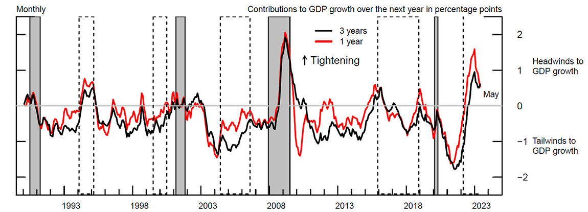
Note: The figure shows the Financial Conditions Impulse on Growth computed with a 1−year and 3−year lookback window, respectively, in red and black. Positive (negative) values of the two indexes denote headwinds (tailwinds) to GDP growth over the next year. The upward arrow indicates the direction of tightening of financial conditions and increasing headwinds to future GDP growth. Gray shaded bars denote periods of recession as dated by the National Bureau of Economic Research: July 1990-March 1991, March 2001-November 2001, December 2007-June 2009, and February 2020-April 2020. The dashed bars represent monetary policy tightening cycles: February 1994-March 1995, July 1999-July 2000, June 2004-August 2006, December 2015-July 2018, March 2022-present. Tightening cycles are defined to start on the month of the first federal funds rate increase and end after the last rate hike.
Source: Haver Analytics; U.S. Census Bureau, Decennial Census of Population and Housing; CoreLogic; Authors' calculations.
One appealing feature of the FCI-G is that its movements can be used to measure whether financial conditions have tightened or loosened, to summarize how changes in financial conditions are associated with real GDP growth over the following year, or both. In this perspective, as indicated by the vertical axis in figure 1, positive (negative) values measure headwinds (tailwinds) to GDP growth over the next year. A zero value means that the cumulative effect on growth of current and past changes in all financial variables sums up to zero, while a reading of 1 percent above (below) the zero line means that financial conditions are a notable headwind (tailwind) to economic activity that is equivalent to a 100 basis point drag (boost) on GDP growth over the following year.
A comparison of the black and red lines in figure 1 highlights the importance of the lags in the propagation of changes in financial conditions through the economy. Focusing on the last two years of data, the figure shows that the degree of tightening estimated with a three-year lookback window (the baseline index) is smaller than what is measured by the index with a one-year lookback window. This difference is due to the highly accommodative conditions that were in place in the aftermath of the COVID-19 pandemic through mid-2021 and that have partly offset the restraining effects on GDP growth associated with higher rates, lower equity prices, and the stronger dollar observed since late 2021. For symmetric reasons, the baseline index has eased less in recent months relative to the index with a one-year lookback window, as the more accommodative conditions observed since the end of 2022 are partly offset by the tighter financial conditions of late 2021 and early 2022. Nevertheless, the most recent readings of the two indexes indicate that financial conditions are estimated to be a drag on GDP growth of roughly 3/4 percentage point over the next year. For historical context, the recent readings of the FCI-G are at their tightest levels since the Global Financial Crisis.
Taking a longer perspective, the FCI-G suggests that financial conditions tend to tighten during a recession (the gray bars) and generally ease in expansions. The index also responds to monetary policy: It typically eases during periods of monetary policy accommodation and tightens over monetary policy tightening cycles (the dashed bars).
Figure 2 compares the FCI-G with the range of financial conditions implied by the indexes developed by Bloomberg, Goldman Sachs, and the Federal Reserve Banks of Chicago, St. Louis, and Kansas City. To facilitate the comparison, each index in figure 2 has been normalized over a common sample period starting in 1990. The vertical axis, therefore, measures the indexes in terms of standard deviations from their own historical averages.
Figure 2. Financial Conditions Impulse on Growth and Other Financial Conditions Indexes
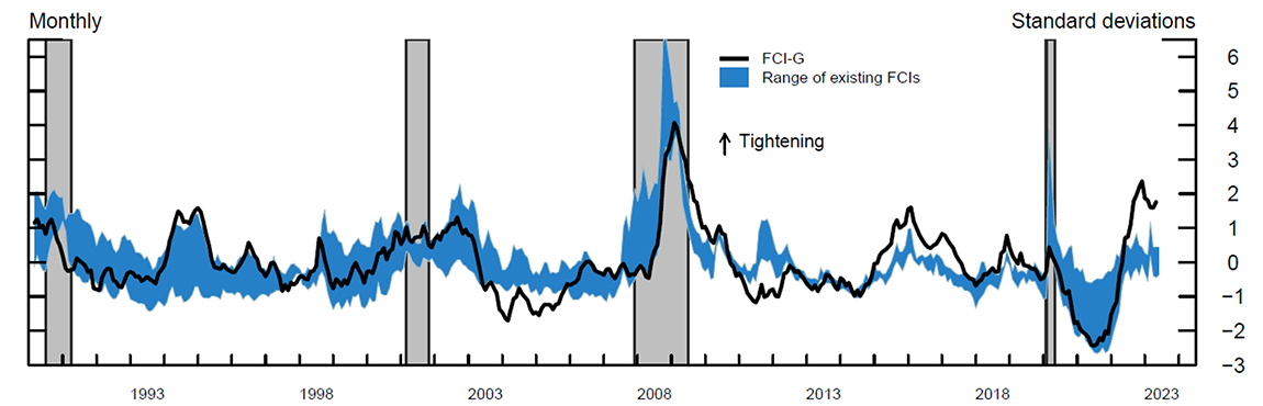
Note: The blue shaded region represents the range of 5 standardized financial conditions indexes (FCIs) developed by Bloomberg, Goldman Sachs, and the Federal Reserve Banks of Chicago, St. Louis, and Kansas City. The upward arrow indicates the direction of tightening of financial conditions. Gray shaded bars denote periods of recession as dated by the National Bureau of Economic Research: July 1990-March 1991, March 2001-November 2001, December 2007-June 2009, and February 2020-April 2020. FCI-G is Financial Conditions Impulse on Growth.
Source: Bloomberg; Federal Reserve Banks of Chicago, St. Louis, and Kansas City; Haver Analytics; U.S. Census Bureau, Decennial Census of Population and Housing; CoreLogic; Authors' calculations.
As shown in the figure, over most of the past three decades, the FCI-G closely tracks changes in broad financial conditions as measured by other FCIs, whose range is represented by the blue shaded region. However, some differences appear, especially during periods of transitory market stress, when the statistical-based FCIs tend to tighten sharply, partly reflecting that some of these indexes are designed to measure stress in financial markets or tend to place larger weights on measures of market volatility. By construction, the FCI-G moves notably when tightening or easing in financial variables are sustained for some time. In recent months, a wedge has appeared between the FCI-G and other FCIs, reflecting the lags through which the rapid and sustained tightening of financial conditions recorded in 2022 acts as a headwind to future GDP growth.
The FCI-G can be broken down across the contributions of each financial variable. These contributions are plotted in figure 3 together with the FCI-G. The decomposition shows that since the end of 2021, the tightening of broad financial conditions has been primarily driven by lower equity prices, higher interest rates (the federal funds rate, mortgage rate, and triple-B corporate bond yield), and the stronger dollar. Moreover, since the second half of last year, the largest headwinds to future growth stem from the changes in short- and long-term interest rates and the dollar, whereas past appreciation in house prices and equity prices recorded over the pandemic continues to be a tailwind to GDP growth.
Figure 3. Financial Conditions Impulse on Growth Components
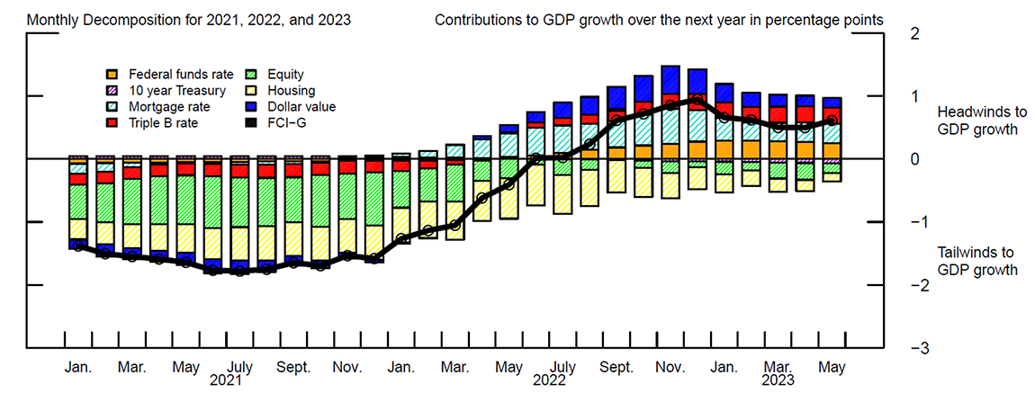
Note: The figure shows the baseline Financial Conditions Impulse on Growth (FCI-G) (black line) and its decomposition into its 7 drivers (the bar charts) over the period that goes from January 2021 through May 2023. Positive (negative) values denote headwinds (tailwinds) to GDP growth over the next year.
Source: Haver Analytics; Authors' calculations.
Technical Appendix
The FCI-G depends on the recent history of three-month changes in seven financial variables: the federal funds rate, the 10-year Treasury yield, the 30-year fixed mortgage rate, the triple-B corporate bond yield, the Dow Jones total stock market index, the Zillow house price index, and the nominal broad dollar index. These variables are available at a daily frequency, except for the Zillow house price index, which is released monthly. See the Data Appendix for additional details.
At any point in time, $$t$$, we partition the lookback window into a number $$T$$ of three-month periods—that is, quarters—indexed by $$i$$, so that the levels of the financial variable $$ j, X_{t}^{j} $$ and $$ X_{t-i}^{j} $$, are observed three months apart from each other when $$i=1$$, six months apart when $$i=2$$, and so on. Across these periods, we compute three-month changes in financial variable $$ X^{j} $$
$$(A.1)\ \Delta X_{t-i}^{j} = X_{t-i}^{j}-X_{t-i-1}^{j} ,\ with\ i=0,1,…,T-1,$$
in which $$X_{t-i}^{j}$$ denotes the level in period $$t-i$$ of the financial variable of interest $$j$$ and $$ \Delta X_{t-i}^{j} $$ denotes its change relative to the level recorded in the preceding three-month period, $$ X_{t-i-1}^{j} $$.
For rates and yields, $$ \Delta X_{t-i}^{j} $$ is calculated as the difference between the average levels of end-of-day values recorded over two subsequent three-month periods. For example, the change in the federal funds rate measured at the end of May 2023 is the difference between the average daily rates in the three-month period between March 1, 2023, and May 31, 2023, and the average daily rates in the three-month period between December 1, 2022, and February 28, 2023. The difference is in levels and therefore expressed in percentage points.
For stock and house price indexes, changes are computed as 100 times three-month differences in log levels and, as such, are expressed in percent rates. For example, the change in the Dow Jones total stock market index measured at the end of May 2023 is 100 times the log difference between the levels of the index on May 31, 2023, and February 28, 2023.
For the dollar index, changes are computed as 100 times three-month differences in log average levels. As such, changes are expressed in percent rates. Average levels are calculated on daily data over three-month periods. For example, the change in the nominal dollar measured at the end of May 2023 is 100 times the log difference between the average daily dollar index in the three-month period between March 1, 2023, and May 31, 2023, and the average daily rate in the three-month period between December 1, 2022, and February 28, 2023
Percent changes in the financial variables of interest are weighted using parameters that reflect the estimated response of GDP to unanticipated permanent changes in those same variables. We sign the weights so that changes in financial variables that tighten financial conditions within the models contribute positively to the index.
We aggregate changes in financial variables using the multipliers $$ \beta_{i}^{j} $$ derived from the public version of the FRB/US model.6
For changes in house prices and in the dollar, the multipliers are computed using other models in use at the Federal Reserve Board. For house prices, the weights are derived from regressions that estimate the role of housing wealth in consumption and of house prices in residential investment. For the nominal dollar index, the weights are based on the effects of an exchange rate appreciation on U.S. GDP, as estimated in the context of the U.S. International Transactions model.7
The multipliers are derived by shocking each of the financial variables separately while holding all other variables constant. This method avoids the issue of potential double counting due to indirect effects working endogenously through the other financial variables.
The multipliers capture how the log level of GDP $$i$$ quarters ahead, $$ GDP_{t+i} $$ deviates from its log trend level, $$ \overline{GDP}_{t+1} $$, following a change in period $$t$$ in the typical financial variable of interest $$j$$, holding fixed all other financial variables in the model:
$$(A.2)\ log(GDP_{t+i}) - log(\overline{GDP}_{t+i}) = \beta_i^j \Delta X_t^j ,\ \text{for}\space i = 0,1,2, \ldots $$
The contribution of $$ \Delta X_t^j $$ to GDP growth can be computed by taking the period-by-period differences in equation (A.2), under the assumption that financial variables do not affect the trend component of GDP.
$$(A.3)\ log(GDP_{t+1+i}) - log(GDP_{t+i}) = (\beta_{i+1}^j - \beta_i^j) \Delta X_t^j,\ \text{for}\space i = 0,1,2,\ldots$$
The contribution of $$ \Delta X_t^j $$ to GDP growth over the subsequent four quarters—that is, one-year-ahead GDP growth—can be obtained by summing equation (A.3) $$ \text{for}\space i = 0,1,2,3, $$ yielding.
$$(A.4)\ log(GDP_{t+4}) - log(GDP_{t}) = ( \beta_{4}^{j} - \beta_{0}^{j}) \Delta X_{t}^{j}. $$
Because the index is computed to evaluate how financial variables contribute to one-year-ahead GDP growth, the weights are set equal to the difference between four-period-ahead and within-period impulse response function coefficients (or multipliers).
Such formulation of the index weights allows us to capture the percent change in the level of real GDP over the following year in response to changes in the financial variables of interest.
Similarly, one-year-ahead GDP growth can be affected by changes in the typical financial variable of interest that occurred in earlier periods, $$ \Delta X_{t-1}^{j} $$ , $$ \Delta X_{t-2}^{j} $$, and so on. To obtain the contribution to GDP growth of all changes in $$ X_t^j $$ within the lookback window of interest (of length $$T$$), the same logic can be applied.
For each period, changes in the typical financial variable $$j$$ —both contemporaneous and past—are translated into contributions to one-year-ahead GDP growth by multiplying them by the corresponding weights:
$$(A.5)\ log(GDP_{t+4}) - log(GDP_{t}) = \Sigma_{i=0}^{T-1} (\beta_{4+i}^{j} - \beta_{0+i}^{j}) \Delta X_{t-i}^{j} $$
The value of the FCI-G is then computed by summing the various contributions across the financial variables of interest and the periods in the lookback window of length $$T$$ according to the following formula:
$$ FCI\mbox{-}G_{t} = log(GDP_{t+4}) - log (GDP_{t}) = \Sigma_{j=1}^7 \Sigma_{i=0}^{T-1} (\beta_{4+i}^{j} - \beta_{0+i}^{j})\Delta X_{t-i}^{j} , $$
in which $$i$$ denotes the number of periods since the occurrence of the change $$ \Delta X^j $$ in financial
variable $$ j, \beta_{0+i}^j $$ and $$ \beta_{4+i}^{j} $$ are the multipliers relative to the effects of financial variable $$j$$ on the log level of real GDP after $$0+i$$ and $$4+i$$ quarters, respectively; and $$T$$ is the length of the lookback window—that is, the number of quarters over which the effects of past changes in financial conditions are cumulated.
Weights used in the computation of the FCI-G with a three-year lookback window are reported in table 1.
Table 1: Weights for the Financial Conditions Impulse on Growth
| Weights | Financial Variables | ||||||
|---|---|---|---|---|---|---|---|
| FFR | 10YT rate | Mortg. rate | Triple B rate | Equity | Housing | Dollar | |
| $$\beta_4 - \beta_0$$ | .09994 | -.00815 | .21743 | .07927 | -.02132 | -.03223 | .048 |
| $$\beta_5 - \beta_1$$ | .06858 | -.01400 | .14525 | .09118 | -.02022 | -.03127 | .048 |
| $$\beta_6 - \beta_2$$ | .05093 | -.01839 | .11905 | .09864 | -.01844 | -.02970 | .045 |
| $$\beta_7 - \beta_3$$ | .03039 | -.02152 | .07750 | .10047 | -.01616 | -.02676 | .039 |
| $$\beta_8 - \beta_4$$ | .02569 | -.02322 | .06243 | .10065 | -.01444 | -.01978 | .031 |
| $$\beta_9 - \beta_5$$ | .02001 | -.02437 | .04514 | .09958 | -.01302 | -.01342 | .023 |
| $$\beta_{10} - \beta_6$$ | .01581 | -.02522 | .03370 | .09766 | -.01175 | -.00605 | .017 |
| $$\beta_{11} - \beta_7$$ | .01135 | -.02591 | .02484 | .09535 | -.01066 | .00077 | .012 |
| $$\beta_{12} - \beta_8$$ | .00739 | -.02640 | .01846 | .09277 | -.00970 | .00424 | .008 |
| $$\beta_{13} - \beta_9$$ | .00396 | -.02670 | .01373 | .09008 | -.00887 | .00667 | .005 |
| $$\beta_{14} - \beta_{10}$$ | .00171 | -.02012 | .00866 | .06654 | -.00634 | .00786 | .002 |
| $$\beta_{15} - \beta_{11}$$ | .00039 | -.01345 | .00490 | .04368 | -.00404 | .00886 | .000 |
Note: The table reports the weights used in the computation of the baseline Financial Conditions Impulse on Growth (FCI-G) index with a three-year lookback window.
Given the sign of the multipliers, positive percent changes in stock and house prices enter the calculation of the FCI-G with a negative sign to capture the feature that increases in these variables reflect easing in financial conditions.
The weights on the 10-year Treasury yield reflect the feature in the FRB/US model that the transmission of changes in long-term rates to real GDP mainly occurs through private long-term rates such as the 30-year fixed mortgage rate and the triple-B corporate bond yield. Following an unanticipated increase in the 10-year Treasury yield, holding private long-term rates fixed, there are no first-order effects on the private-expenditure components of GDP as private rates have not changed. Instead, because of the implied higher coupon payments to bondholders in the private sector, an increase in the 10-year Treasury yield entails a small positive income effect, which is equivalent to an easing in financial conditions.
The y-axis scale in figure 1 displays the FCI-G in terms of tailwinds and headwinds for GDP growth over the following year.
In this note, we report a monthly version of the FCI-G. Using the same methodology and with limited data adjustments, we can compute weekly or daily versions of this index.
Figure 4 displays the history of the FCI-G with one-year and three-year lookback window starting in January 1979, respectively in red and black.
Figure 4. Financial Conditions Impulse on Growth over a Longer Sample Period
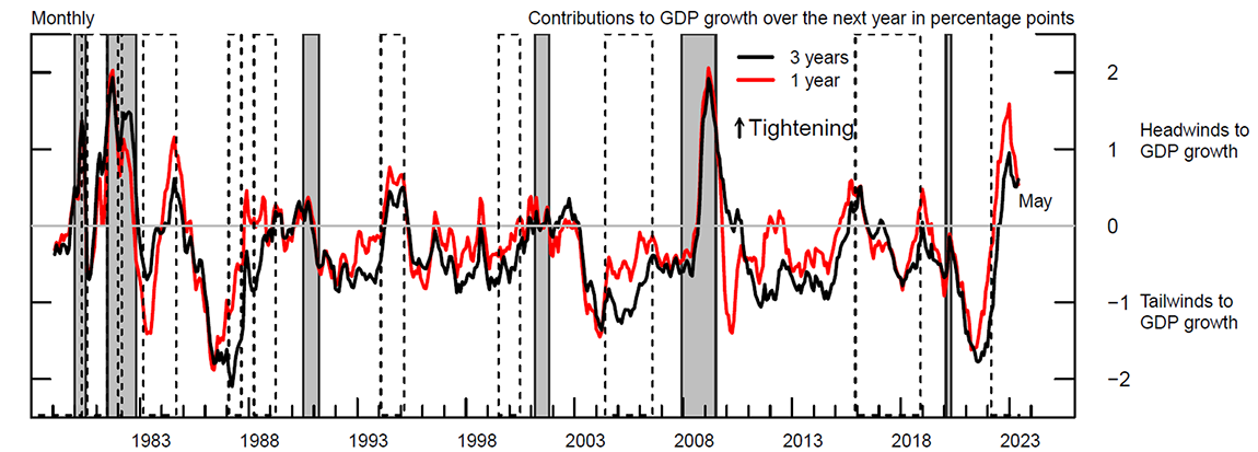
Note: The figure shows the Financial Conditions Impulse on Growth computed with a 1-year and 3-year lookback window, respectively, in red and black. Positive (negative) values of the two indexes denote headwinds (tailwinds) to GDP growth over the next year. The upward arrow indicates the direction of tightening of financial conditions and increasing headwinds to future GDP growth. Gray shaded bars denote periods of recession as dated by the National Bureau of Economic Research: January 1980-July 1980, July 1981-November 1982, July 1990-March 1991, March 2001-November 2001, December 2007- June 2009, and February 2020-April 2020. The dashed bars represent monetary policy tightening cycles: February 1977-May 1980, August 1980-July 1981, January 1982-March 1982, March 1983-September 1984, February 1987-September 1987, April 1988-April 1989, February 1994-March 1995, July 1999-July 2000, June 2004-August 2006, December 2015-July 2018, March 2022-present. Tightening cycles are defined to start on the month of the first federal funds rate increase and end after the last rate hike.
Source: Haver Analytics; U.S. Census Bureau, Decennial Census of Population and Housing; CoreLogic; Authors' calculations.
Data Appendix
1. The federal funds rate
Federal funds (effective): Federal Reserve Board, Statistical Release H.15, "Selected Interest Rates (Daily)," Unique ID: RIFSPFF_N.B (https://www.federalreserve.gov/releases/h15/default.htm).
Haver Analytics: FFED@DAILY
Federal Reserve Economic Data (FRED): Federal Funds Effective Rate (DFF: https://fred.stlouisfed.org/series/DFF).
Effective Federal Funds Rate: Federal Reserve Bank of New York, reference rates (https://www.newyorkfed.org/markets/reference-rates).
Haver Analytics: FFEDTA@DAILY
FRED: Effective Federal Funds Rate (EFFR: https://fred.stlouisfed.org/series/EFFR).
2. The 10-year Treasury yield
Ten-year coupon-equivalent par yield: Federal Reserve Board, Nominal Yield Curve (Daily), Unique ID: SVENPY10 (https://www.federalreserve.gov/data/nominal-yield-curve.htm).8
Haver Analytics: FYCEPA@DAILY
3. The 30-year fixed mortgage rate
From December 30, 2016, to present: Optimal Blue LLC. Optimal Blue Mortgage Price Data (https://www2.optimalblue.com/obmmi/): 30-Year Fixed Rate Conforming Mortgage Index, adjusted for average points and fees paid by prime borrowers at origination.
From February 2, 1976, to December 29, 2016: Weekly average rate on 30-year fixed-rate mortgages, Freddie Mac, Primary Mortgage Markey Survey (https://www.freddiemac.com/pmms).
Haver Analytics: FRM30@SURVEYS
FRED: 30-Year Fixed Rate Mortgage Average in the United States (MORTGAGE30US: https://fred.stlouisfed.org/series/MORTGAGE30US).
4. The triple-B corporate bond yield
From January 2, 1997, to present:
ICE Bank of America (BofA) triple-B U.S. Corporate Index (C0A4), effective yield (https://indices.theice.com/).
Haver Analytics: FMLC3B@DAILY
FRED: ICE BofA triple-B U.S. Corporate Index Effective Yield (BAMLC0A4CBBBEY: https://fred.stlouisfed.org/series/BAMLC0A4CBBBEY).
From January 3, 1989, to December 31, 1996:
ICE BofA triple-B U.S. Corporate Index (C0A4), Yield to Maturity (https://indices.theice.com/).
Haver Analytics: FMLC3BM@DAILY
From February 1976 to December 1988:
Monthly yields computed from end-of-month secondary-market prices for corporate bonds from the Lehman-Warga fixed-income database using the Nelson-Siegel (1987) yield-curve model, as detailed in Gilchrist and Zakrajšek (2012).
5. The Dow Jones total stock market index
From January 2, 1987, to present: Dow Jones U.S. Total Stock Market Index
Haver Analytics: SPTSMF@DAILY
From December 3, 1979 to December 31, 1986: Wilshire 5000 Full Cap Price Index
Haver Analytics: SPWI@DAILY
Fred: Wilshire 5000 Full Cap Price Index (WILL5000PRFC: https://fred.stlouisfed.org/series/WILL5000PRFC).
From February 1976 to November 1979: authors' calculations based on the interpolation of monthly values for the Wilshire 5000 with daily values for the S&P 500 (Haver Analytics: SP500@DAILY).
6. The Zillow house price index
From January 2000 to present: Zillow Home Value Index (ZHVI) for all homes (https://www.zillow.com/research/data/)
Haver Analytics: USZHV@USECON
FRED: Zillow Home Value Index (USAUCSFRCONDOSMSAMID: https://fred.stlouisfed.org/series/USAUCSFRCONDOSMSAMID).
From February 1976 to December 1999: An approximation of the ZHVI is constructed by taking county-level annual estimates for housing stocks and median house values from the Decennial Census of Population and Housing. The annual estimates are then interpolated using the corresponding county-level monthly CoreLogic house price indexes excluding distressed sales. Finally, for each month, the implied county-level home values are aggregated following the ZHVI methodology as closely as possible.
7. The nominal broad dollar index
From January 2, 2006, to present: Nominal Broad Dollar Index - Daily Index: Federal Reserve Board, Foreign Exchange Rates - H.10, Unique ID: JRXWTFB_N.B (https://www.federalreserve.gov/releases/h10/summary/jrxwtfb_nb.htm).
FRED: Nominal Broad U.S. Dollar Index (DTWEXBGS: https://fred.stlouisfed.org/series/DTWEXBGS).
From February 2, 1976, to December 30, 2005: Haver Analytics: FXTWBDI@DAILY
References
Brayton, Flint, Thomas Laubach, and David Reifschneider (2014). "The FRB/US Model: A Tool for Macroeconomic Policy Analysis," FEDS Notes. Washington: Board of Governors of the Federal Reserve System, April 3, https://doi.org/10.17016/2380-7172.0012.
Gilchrist, Simon, and Egon Zakrajšek (2012). "Credit Spreads and Business Cycle Fluctuations," American Economic Review, vol. 102 (June), pp. 1692–720, http://dx.doi.org/10.1257/aer.102.4.1692.
Gruber, Joseph, Andrew McCallum, and Robert Vigfusson (2016). "The Dollar in the U.S. International Transactions (USIT) Model," IFDP Notes. Washington: Board of Governors of the Federal Reserve System, February 8, https://doi.org/10.17016/2573-2129.16.
Gürkaynak, Refet S., Brian Sack, and Jonathan H. Wright (2007). "The U.S. Treasury Yield Curve: 1961 to the Present," Journal of Monetary Economics, vol. 54 (November), pp. 2291–304, https://doi.org/10.1016/j.jmoneco.2007.06.029.
Laforte, Jean-Philippe (2018). "Overview of the Changes to the FRB/US Model (2018)," FEDS Notes. Washington: Board of Governors of the Federal Reserve System, December 7, https://doi.org/10.17016/2380-7172.2306.
Nelson, Charles R., and Andrew F. Siegel (1987). "Parsimonious Modeling of Yield Curves," Journal of Business, vol. 60 (October), pp. 473–89, http://www.jstor.org/stable/2352957.
Svensson, Lars E.O. (1994). "Estimating and Interpreting Forward Interest Rates: Sweden 1992–1994," NBER Working Paper Series 4871. Cambridge, Mass.: National Bureau of Economic Research, September, https://doi.org/10.3386/w4871.
Svensson, Lars E.O. (1995). "Estimating Forward Interest Rates with the Extended Nelson and Siegel Method," Sveriges Riksbank Quarterly Review, no. 3, pp. 13–26.
1. We thank Elliot Anenberg, Hess Chung, Andrea De Michelis, Eric Fischer, Colin Hottman, Paul Lengermann, Logan Lewis, David López-Salido, Andrew Paciorek, Francisco Palomino, Michael Palumbo, and Seth Searls for many helpful conversations and feedback. At various stages of this project, Greg Marchal, Makena Schwinn, and Diego Silva provided excellent support. The analysis and conclusions set forth are those of the authors and do not indicate concurrence by the Board of Governors of the Federal Reserve System. Any errors or omissions are the responsibility of the authors. Return to text
2. Starting February 2025, an update of this index will be posted at 10:00 a.m. on the 20th day of each month, or on the closest business day following the 20th of each month. Previously, the update of this index was posted at 10:00 a.m. on the 15th day of each month, or on the closest business day following the 15th of each month. In situations when the scheduled release falls during the Federal Open Market Committee communications blackout period, the updated index will be posted after the blackout period has ended. On the rare occasion when source data become unavailable or delayed, the publication of the updated index will be delayed. The update will include both monthly and quarterly time series, to reflect values up to the closest month- and quarter-end. Because the index is a research product and not an official statistical release, it is subject to delay, revision, or methodological changes without advance notice. As an experimental series, the index may be discontinued at any time. Accordingly, it should be used for informational purposes only. The Board of Governors of the Federal Reserve System and its staff will not be liable for any damages arising out of, or in connection with, the use of the index. Return to text
3. For more information about the FRB/US model—a large-scale estimated model of the U.S. economy—see https://www.federalreserve.gov/econres/us-models-about.htm. For a description of the quantitative model used to assess the role of the nominal broad dollar index on the U.S. economy, see Gruber, McCallum, and Vigfusson (2016). Return to text
4. Nearly all weights associated with changes in financial variables that occurred outside the three-year window are equal to zero. Return to text
5. Three additional assumptions made in the construction of the FCI-G are worth noting. First, the index embeds the assumption that the multipliers are fixed over time. Second, there is some uncertainty around the estimated multipliers that is not reflected in the computation of the FCI-G. Third, while the financial variables included in the index are all in nominal terms, a real version of the index can be constructed without meaningfully altering the interpretation and the historical evolution of the FCI-G. Return to text
6. For detailed descriptions of the FRB/US model, see Brayton, Laubach, and Reifschneider (2014) and Laforte (2018). Return to text
7. As discussed in Gruber, McCallum, and Vigfusson (2016), the U.S. International Transactions model is one of a suite of quantitative models used at the Federal Reserve Board to assess the dollar's effect on the U.S. economy. Return to text
8. The estimated 10-year Treasury yield is based on the work of Svensson (1994, 1995) and Gürkaynak, Sack, and Wright (2007). Return to text
Ajello, Andrea, Michele Cavallo, Giovanni Favara, William B. Peterman, John Schindler, and Nitish R. Sinha (2023). "A New Index to Measure U.S. Financial Conditions," FEDS Notes. Washington: Board of Governors of the Federal Reserve System, June 30, 2023, https://doi.org/10.17016/2380-7172.3281.
Disclaimer: FEDS Notes are articles in which Board staff offer their own views and present analysis on a range of topics in economics and finance. These articles are shorter and less technically oriented than FEDS Working Papers and IFDP papers.