FEDS Notes
May 05, 2017
Measuring the Severity of Stress-Test Scenarios
Bora Durdu, Rochelle Edge, and Daniel Schwindt
Unfavorable macroeconomic and financial scenarios are a core element of bank stress tests, and the degree to which variables deteriorate in a scenario--i.e., the scenario's severity--is a central design feature of any stress test exercise.1 This note presents a simple methodology for measuring the severity of stress-test scenarios, which relies on a comparison of scenario developments with historically stressful episodes--specifically, recessions and house-price retrenchments. This methodology is outlined in section 1. Section 2 then applies this methodology to the last few years of the Federal Reserve Board's Comprehensive Capital Analysis and Review (CCAR) stress scenarios. Doing so demonstrates one of the benefits of having a simple measure of scenario severity--namely, it allows for scenario severity to be compared across time. Performing such a comparison should also help prevent a potential downside of stress testing, which is that stress testing can add to existing financial pro-cyclicality by specifying scenarios that are less severe when the economy is strong and more severe when the economy is weak. Indeed, scenarios should become more severe when the economy is strong, since under these conditions financial-system vulnerabilities build-up, which, in turn, raises the risk of more severe cyclical downturns.2 Section 3 concludes by noting some limitations associated with our methodology and by discussing alternative--albeit more complicated--approaches that may also address these limitations. The section also discusses other situations in which it may be useful to have a simple severity measure to make comparisons across scenarios.
1. Measuring severity based on historical episodes
Our methodology first measures the severity of key individual scenario variables and then aggregates these variable-specific measures into broader measures. In developing our measures, we focus on a number of key scenario variables--specifically, real gross domestic product (GDP), the unemployment rate, house prices, equity prices, the VIX (an index of implied volatility), and triple-B spreads. We begin the description of our methodology by explaining how the severity of unfavorable developments in real GDP and the unemployment rate is assessed. The methodology is similar for the other variables we consider.
1.1. Measuring the severity of real-activity scenario variables
Our approach is to compare how variables evolve in the scenarios with how the same variables evolved in historically stressful episodes. For real GDP and the unemployment rate, historically stressful episodes are past recessions. We limit ourselves to the last nine post-war U.S. recessions, as defined by the National Bureau of Economic Research (NBER) Business Cycle Dating Committee. Table 1 documents the behavior of real GDP and the unemployment rate over these recessionary periods. We also provide a qualitative classification of the severity of each recession, with a recession being classified as either mild, moderate, or severe.3 As Table 1 shows, the four recessions in which real GDP declined 2-1/2 percent or more and the unemployment rate increased 3 percentage points or more are classified as severe recessions. The two recessions before the most recent one, both of which featured the unemployment rate increasing less than 1-1/4 percent, are classified as mild recessions. The remaining three recessions, which fall in between these extremes, are classified as moderate recessions. In Table 1, we show the measures for the 2007-09 recession, known as the Great Recession, and for the average of the mild recessions in bold. Our severity measures key off the developments in these recessions.
Table 1. U.S. Recessions Characteristics
| Peak | Trough | Severity | Duration (quarters) | During the Recession | Including after the Recession | ||
|---|---|---|---|---|---|---|---|
| Change in Real GDP (percent) | Change in the Unemployment Rate (p.p.) | Change in the Unemployment Rate (p.p.) | Peak Unemployment Rate (p.p.) | ||||
| 1957:Q3 | 1958:Q2 | Severe | 4 | -3.6 | 3.1 | 3.1 | 7.4 |
| 1960:Q2 | 1961:Q1 | Moderate | 4 | -1 | 1.6 | 1.8 | 7.0 |
| 1969:Q4 | 1970:Q4 | Moderate | 5 | -0.2 | 2.3 | 2.5 | 6.0 |
| 1973:Q4 | 1975:Q1 | Severe | 6 | -3.1 | 3.5 | 4.1 | 8.9 |
| 1980:Q1 | 1980:Q3 | Moderate | 3 | -2.2 | 1.4 | 1.4 | 7.7 |
| 1981:Q3 | 1982:Q4 | Severe | 6 | -2.8 | 3.3 | 3.3 | 10.7 |
| 1990:Q3 | 1991:Q1 | Mild | 3 | -1.3 | 0.9 | 1.9 | 7.6 |
| 2001:Q1 | 2001:Q4 | Mild | 4 | 0.2 | 1.3 | 1.9 | 6.2 |
| 2007:Q4 | 2009:Q2 | Severe | 7 | -4.2 | 4.5 | 5.1 | 9.9 |
| Average | -- | Severe | 6 | -3.4 | 3.6 | 3.9 | 9.2 |
| Average | -- | Moderate | 4 | -1.1 | 1.8 | 1.9 | 6.9 |
| Average | -- | Mild | 4 | -0.6 | 1.1 | 1.9 | 6.9 |
Source: Bureau of Economic Analysis (BEA); Bureau of Labor Statistics (BLS).
For real GDP, the severity measure takes a score of 100 if the maximum decline in real GDP during the scenario equals the 4.2 percent decline that occurred during the Great Recession, and takes a score of 0 if the maximum decline equals the 0.6 percent decline that occurred, on average, across mild recessions. Real GDP scenario paths that decline by other maximum amounts are scored according to a simple linear interpolation and extrapolation. In particular, the linear equation that connects the two points $$\downarrow GDP$$ = 4.2 and $$Score_{\downarrow GDP}=$$ 100 and $$\downarrow GDP$$ = 0.6 and $$Score_{\downarrow GDP}=$$ 0, specifically,
$$$$Score_{\downarrow GDP}=-26.1*\downarrow GDP-10.8, $$$$
scores the declines in all other real GDP scenario paths.
In a weakening labor market, both the increase in the unemployment rate in the scenario and the level to which the unemployment rate rises may be stressful to banks. In considering unemployment rate path severity, we therefore consider both a "changes" severity measure, and a "levels" measure. In computing the changes measure, we follow a similar procedure to what we used for GDP by measuring the severity of the increase in the unemployment rate, albeit focusing on the full increase in the unemployment rate associated with the recession rather than just on the increase over the recessionary quarters. In particular, the linear equation that connects the two points $$\ \uparrow UR$$ = 5.1 and $$Score_{\uparrow UR}$$ = 100 and $$\ \uparrow UR$$ = 1.9 and $$Score_{\uparrow UR}$$ = 0, specifically,
$$$$Score_{\uparrow UR}=31.8*\ \uparrow UR-61.9, $$$$
scores the increases in unemployment rate scenario paths. For the levels measure, the linear equation that connects the two points of $$MAX\left(UR\right)$$ = 9.9 and $$Score_{MAX\left(UR\right)}$$ = 100 and $$MAX\left(UR\right)$$ = 6.9 and $$Score_{MAX\left(UR\right)}$$ = 0, specifically,
$$$$Score_{MAX\left(UR\right)}=100*\frac{MAX\left(UR\right)-6.9}{9.9-6.9} $$$$
scores the peak levels in the unemployment rate scenario paths.
We obtain an overall real-activity severity score by averaging the three individual real-activity scores, specifically,
$$$$Overall\ Score_{Real\ Activity}=\frac{Score_{\downarrow GDP}+Score_{\uparrow UR}+Score_{MAX(UR)}}{3} $$$$
1.2. Measuring the severity of house-price scenario variables
While for real GDP and the unemployment rate historically stressful episodes are past NBER-identified U.S. recessions, this is not the case for house prices, which have increased in many U.S. recessions. Therefore, we define "housing recessions" to be stressful episodes for house prices and identify these episodes to be when the ratio of the House Price Index to Per Capita Disposable Personal Income (HPI-to-DPI) experiences sustained declines. These episodes are shown by the three gray shaded areas in Figure 1 and correspond broadly to episodes during which real residential investment expenditures also experienced sustained declines, as shown by three gray shaded areas in Figure 2. The precise contractionary periods for the two series are, however, different. Hence, were housing recessions to be classified based not only on house-price retrenchments, we would likely have arrived at slightly different timings of housing recessions.4
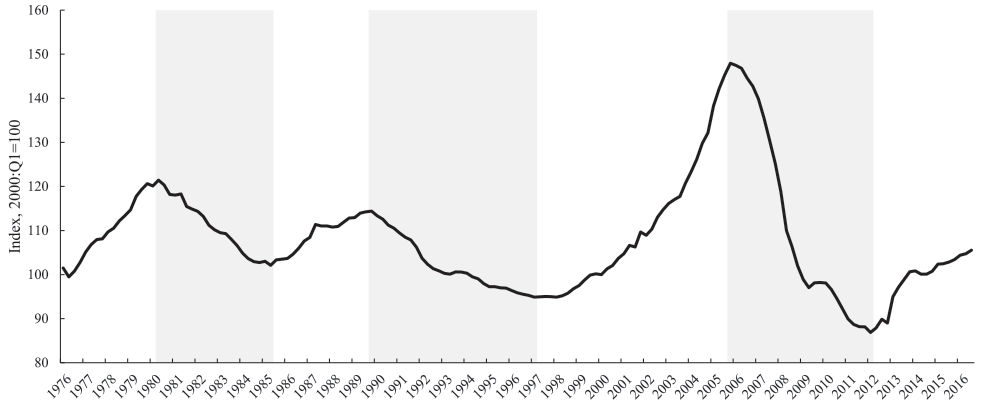
Note: Gray shaded regions define the periods of the peak through the trough in the HPI-to-DPI ratio; these periods are 1980:Q2–1985:Q2, 1989:Q4–1997:Q1, and 2005:Q4–2012:Q1.
Source: CoreLogic; BEA.
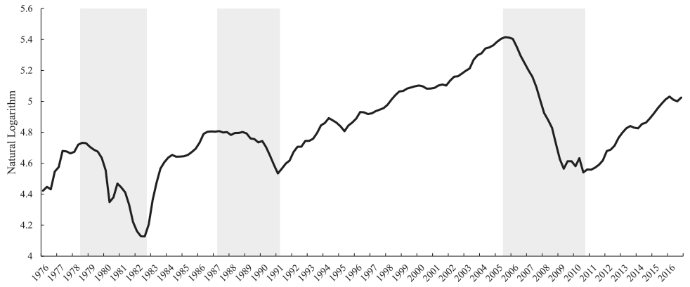
Note: Gray shaded regions define the periods of the peak through the trough in the natural logarithm of RRI; these periods are 1978:Q3–1982:Q3, 1987:Q2–1991:Q1, and 2005:Q3–2010:Q3.
Source: BEA.
Table 2 reports the changes in the nominal House Price Index as well as the changes and the trough level in the HPI-to-DPI ratio in the three identified housing recessions. The first housing recession in our sample occurred during the early 1980s, with about a 16 percent peak-to-trough decline in the HPI-to-DPI ratio. The next housing recession in our sample features a broadly similar-sized HPI-to-DPI decline. Given the reasonable-sized magnitudes and durations of these HPI-to-DPI declines, we consider these housing recessions to be moderate. The most severe housing recession occurred during the recent Great Recession, with a peak-to-trough decline in the HPI-to-DPI ratio of around 40 percent.
Table 2. House Price Recessions Characteristics
| Peak | Trough | Severity | Duration (quarters) | Change in HPI (percent) | Change in HPI-to-DPI (percent) | HPI-to-DPI Trough Level (2000:Q1 = 100) |
|---|---|---|---|---|---|---|
| 1980:Q2 | 1985:Q2 | Moderate | 20 | 26.6 | -15.9 | 102.1 |
| 1989:Q4 | 1997:Q1 | Moderate | 29 | 10.5 | -17.0 | 94.9 |
| 2005:Q4 | 2012:Q1 | Severe | 25 | -29.6 | -41.3 | 86.9 |
| Average | -- | Moderate | 25 | 18.5 | -16.5 | 98.5 |
Note: The first two columns show the peak and trough dates for the HPI-to-DPI ratio.
Source: CoreLogic; BEA.
The adverse house-price developments reported in Table 2 form the basis for our severity measure for scenario house-price paths. Accordingly, the severity measure takes a score of 100 if the decline in the nominal HPI, the decline in the HPI-to-DPI ratio, and the trough level of the HPI-to-DPI ratio are similar to those that occurred in the 2005--12 housing recession. Since the remaining housing recessions in our sample are not mild recessions, we do not assign a score of 0 to their average. Rather we assign a score of 6.0, which is the same value as the overall severity score for real-activity variables in moderate recessions. These specifications imply the following scoring equations for house-price variables:
$$$$Score_{\downarrow HPI}=\left(-1.9\right)*\downarrow HPI+42.8, $$$$
$$$$Score_{\downarrow HPI-DPI}=\left(-3.9\right)*\downarrow \left(HPI / DPI\right)-56.5, \text{and} $$$$
$$$$Score_{MIN(HPI-DPI)}=\frac{85.4-MIN\left(HPI / DPI\right)}{85.4-59.7} $$$$
Our motivation for using both the change and the trough level of the HPI-to-DPI ratio in our measures of scenario severity is the same as our motivation for using both the change and peak level of the unemployment rate. That is, in a weakening housing market, both the decline in house prices and the level to which house prices fall are likely stressful to banks.
We obtain an overall house-price severity score by averaging the individual scores, specifically,
$$$$Overall\ Score_{House\ Prices}=\frac{Score_{\downarrow HPI}+Score_{\downarrow (HPI / DPI)}+Score_{MAX(HPI / DPI)}}{3} $$$$
1.3. Measuring the severity of financial market scenario variables
In contrast to housing, historically stressful financial market episodes coincide more closely with NBER recession timings, although their precise timing still differs by a couple of quarters. Table 3 reports developments in equity prices, triple-B spreads, and the VIX in historically stressful financial-market episodes that we also categorize as being mild, moderate or severe. In all cases, these classifications correspond to those for the similarly timed NBER recession.
In our scoring equations, the decline in equity prices, the increase in triple-B spreads, and the level to which the VIX rose in the Great Recession are assigned scores of 100, while developments for these variables in mild recessions are assigned scores of 0. These specifications imply the following scoring equations for financial-market variables.
$$$$Score_{\downarrow Equity\ Prices}=-3.4*\downarrow Equity\ Prices-58.43, $$$$
$$$$Score_{\uparrow BBB\ Spread}=0.3*\uparrow BBB\ Spread-15.5, $$$$
$$$$Score_{VIX}=100*\frac{VIX-40.1}{80.9-40.1} $$$$
We obtain an overall financial-market severity score by averaging the individual scores, specifically,
$$$$Overall\ score_{Financial\ Markets}=\frac{Score_{\downarrow Equity\ Prices}+Score_{\uparrow BBB\ Spread}+Score_{VIX}}{3} $$$$
Table 3. U.S. Recession Financial Characteristics
| Start | End | Severity | Duration (quarters) | Peak Level of VIX | Change in BBB Spread (bps) | Change in S 500 Index (percent) |
|---|---|---|---|---|---|---|
| 1957:Q3 | 1958:Q2 | Severe | 4 | -- | -- | -12.6 |
| 1960:Q2 | 1961:Q1 | Moderate | 4 | -- | -- | -6.2 |
| 1969:Q4 | 1970:Q4 | Moderate | 5 | -- | -- | -24.3 |
| 1973:Q4 | 1975:Q1 | Severe | 6 | -- | 269.2 | -33.8 |
| 1980:Q1 | 1980:Q3 | Moderate | 3 | -- | 160.6 | 0.6 |
| 1981:Q3 | 1982:Q4 | Severe | 6 | -- | 107.4 | -14.8 |
| 1990:Q3 | 1991:Q1 | Mild | 3 | 36.5 | 41.0 | -8.9 |
| 2001:Q1 | 2001:Q4 | Mild | 4 | 43.7 | 76.5 | -23.7 |
| 2007:Q4 | 2009:Q2 | Severe | 7 | 80.9 | 438.4 | -47.6 |
| Average | -- | Severe | 5.8 | 80.9 | 271.7 | -27.2 |
| Average | -- | Moderate | 4.0 | -- | 160.6 | -10.0 |
| Average | -- | Mild | 3.5 | 40.1 | 58.8 | -16.3 |
Note: First two columns denote the start and end of the nine postwar U.S. recessions as defined by the NBER. The values in the last three columns are associated with the recessions but do not necessarily follow the same timing as the NBER definitions.
Source: BofA Merrill Lynch Global Research, Bond Indices; Chicago Board Options Exchange (CBOE); Global Financial Data, https://www.globalfinancialdata.com/index.html; Standard & Poor's, S&P 500 Index, accessed via Bloomberg.
2. Recession measure results
Figure 3 presents our severity score measures based on the paths of real activity, house prices, and financial market variables for CCAR 2013 to CCAR 2017.5 In each case, we first report the overall severity measure--shown in the left panel in each row of charts--followed by the three component measures--shown in the remaining panels in the row.
As the upper left panel of Figure 3 shows, the severity of CCAR scenarios when considered in terms of real-activity variables edged down between CCAR 2013, CCAR 2014, and CCAR 2015 but then increased in CCAR 2016 and CCAR 2017. Declining peak unemployment rates accounted for all of the reduction between CCAR 2013 and CCAR 2015 in overall real-activity scenario severity and increases in the changes in GDP and the unemployment rate accounted for all of the increase in scenario severity in CCAR 2016 and CCAR 2017. This latter development reflects the fact that in CCAR 2016, the key element of CCAR scenario design that attempts to limit the pro-cyclicality began to take effect.6 Also note that overall real-variable severity remained close to the Great Recession benchmark level for CCAR 2013 to CCAR 2015 but then rose above this level in CCAR 2016 and CCAR 2017.
As the middle left panel of Figure 3 shows, the severity of CCAR house-price scenario variables increased between CCAR 2013 and CCAR 2014 and then edged down slightly in subsequent CCAR rounds. The increase in severity between CCAR 2013 and CCAR 2014 reflects the increase in the absolute size of the decline in the nominal HPI in CCAR 2014, which was specified in the scenario so as to reverse some of the large house price gains that occurred over the year preceding the scenario's release.7 The edging down of severity between CCAR 2014 and CCAR 2017 reflects increases in the trough levels of the HPI-to-DPI ratio that have occurred as house prices have increased. In contrast to the overall real-variable severity score, the overall house-price severity score is consistently lower than the Great Recession benchmark. This outcome reflects the fact that none of the HPI or HPI-to-DPI declines specified in CCAR scenarios to date have been as large as the decline that occurred in the Great Recession.
As the lower-left panel of Figure 3 shows, the severity of the financial variables in the CCAR scenarios has not exhibited any persistent trends, on aggregate, over the past few years. The increase in severity between CCAR 2014 and CCAR 2015 reflects the larger widening of corporate bond spreads in CCAR 2015 that also had implications for equity prices and the VIX.8 This specific development was not featured in subsequent scenarios, and, as a result, the severity of financial variables diminished with CCAR 2016 and CCAR 2017. This decrease in severity has, however, been tempered by the real economy weakening by more in the two most recent scenarios and the implications that this weakening has for financial variables.
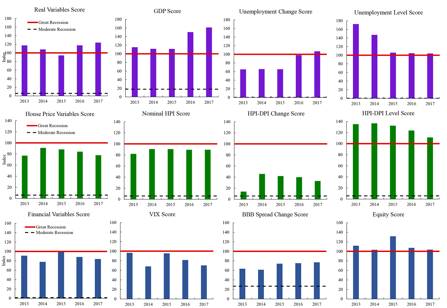
Note: Figures in leftmost column are computed by taking a simple average of the scores shown in the other three charts in the same row. Thick red line represents the score of the financial or housing crisis. Dashed black line shows the score a moderate recession would receive.Year labels represent the CCAR cycles. A score of 100 means a scenario is as severe as the Great Recession, while a score of 0 signifies a scenario as severe as the average U.S mild recession. VIX Score does not contain a moderate recession line because of data restrictions.
Source: Staff estimates from public CCAR release and historical data from BEA, BLS, Wall Street Journal, Chicago Board Options Exchange (CBOE), Global Financial Data, https://www.globalfinancialdata.com/index.html; BofA Merrill Lynch Global Research, Bond Indices; Standard & Poor's, S&P 500 Index, accessed via Bloomberg.
3. Discussion
The main strength of our methodology for measuring stress-test scenario severity is its simplicity. That is, it translates a number of the scenario variable paths published each year at the start of the CCAR cycle into the simple scores shown in Figure 3, which in turn, can be compared across scenarios and against historical stressful episodes. However, our methodology has limitations; hence, it should not be used as the sole measure of scenario severity.
One limitation of our methodology is that, while the scores are interpretable in terms of the past macroeconomic outcomes, they are not interpretable in terms of the stress they imply to banks. One way to obtain scores that are interpretable in terms of stresses to banks is to consider what scenario variable paths imply for relevant bank-performance measures. For example, one could combine the paths of scenario variables with equations projecting key bank performance measures--like the net charge-offs models developed by Guerrieri and Welch (2012)--and determine scenario severity scores based on the overall levels of net charge-offs that result. Using such models would also address another issue with our severity score measures, namely, they assess severity based on the maximum absolute change or the peak or trough level to which a variable deteriorates in the scenario without considering for how long the variable remains at an extreme value. A downside of this alternative approach to gauging severity is that is loses the simplicity of our measure. Additionally, for comparisons of scenario severity over time, the projection jump-off point could influence measured scenario severity as much as the scenario itself.
Finally, note that the variables for which we have developed scenario scoring methodologies are variables that are more closely related to losses on bank assets. Additional variables are also important for pre-provision net revenue (PPNR), which is also a significant bank-income variable in stress testing.9 In principal, simple severity score measures could be formulated for the variables that drive the components of PPNR, although a methodology that uses forecasting models--similar to that described above for net charge-offs--represents another potential approach.
The aforementioned limitations do not diminish the value of our methodology; rather, they suggest that our measures should be complemented with other methodologies for gauging scenario severity. Finally, our methodology for comparing scenario severity has applications beyond just the example presented in this note. Our methodology can be used to compare the severity of scenarios specified by different banks or financial institutions in horizontal company-run stress testing exercises as well as to compare severity across the scenarios specified by different national authorities in their own stress testing exercises.
4. References
Board of Governors of the Federal Reserve System (2013a). "Policy Statement on the Scenario Design Framework for Stress Testing," final rule (Docket No. OP-1452), Federal Register, vol. 78 (November 29), pp. 71435–48.
-------- (2013b). 2014 Supervisory Scenarios for Annual Stress Tests Required under the Dodd-Frank Act Stress Testing Rules and the Capital Plan Rule. Washington: Board of Governors, November, https://www.federalreserve.gov/bankinforeg/bcreg20131101a1.pdf.
-------- (2014). 2015 Supervisory Scenarios for Annual Stress Tests Required under the Dodd-Frank Act Stress Testing Rules and the Capital Plan Rule. Washington: Board of Governors, October, https://www.federalreserve.gov/newsevents/press/bcreg/bcreg20141023a1.pdf.
Guerrieri, Luca, and Michelle Welch (2012). "Can Macro Variables Used in Stress Testing Forecast the Performance of Banks?" Finance and Economics Discussion Series 2012-49. Washington: Board of Governors of the Federal Reserve System, July, https://www.federalreserve.gov/pubs/feds/2012/201249/201249pap.pdf.
Hirtle, Beverly, and Andreas Lehnert (2015). "Supervisory Stress Tests," Annual Review of Financial Economics, vol. 7, pp. 339–55.
Tarullo, Daniel K. (2012). "Developing Tools for Dynamic Capital Supervision," speech delivered at the Federal Reserve Bank of Chicago Annual Risk Conference, Chicago, April 10, https://www.federalreserve.gov/newsevents/speech/tarullo20120410a.htm.
1. See Hirtle and Lehnert (2015) for a discussion of the key design features of stress tests, including scenario specification. Return to text
2. For a detailed discussion of the issue of stress-test scenario severity and financial-system pro-cyclicality, see Board of Governors' (2013a). Return to text
3. These classifications, which are based on developments in real GDP and the unemployment rate, are the same as those reported in Table 1 of the Board of Governors' (2013a). Note that these are not NBER-defined categorizations. Return to text
4. Our preference for focusing solely on the HPI-to-DPI ratio to identify historically stressful periods for the housing sector is that both the HPI and DPI are variables included in the Federal Reserve Board's CCAR stress scenarios, and, ultimately, we apply our methodology to these scenarios. Another ratio that could be used to identify stressful periods for the housing sector is the house-price-to-rent ratio. Return to text
5. We begin our evaluation of scenario severity with CCAR 2013 since it was for this CCAR round that the Federal Reserve Board began following the methodology laid out in the (then-proposed) methodology described in Board of Governors (2013a). Return to text
6. The element that limits the pro-cyclicality boosts the scenario's unemployment rate increase when the actual level of the unemployment rate fall to low levels. In Board of Governors (2013a), the unemployment rate is specified to increase by between 3 and 5 percentage points from its initial level--with the typical increase being 4 percentage point--with the stipulation that if such an increase does not raise the level of the unemployment rate to at least 10 percent, the path of the unemployment rate will be specified so as to raise the unemployment rate to that level. Return to text
7. For a discussion of this change, see Board of Governors (2013b). Return to text
8. For a discussion of this change, see Board of Governors (2014). Return to text
9. See, Tarullo (2012) for a discussion of the importance of also projecting PPNR paths in stress testing. Return to text
Durdu, Bora, Rochelle Edge, and Daniel Schwindt (2017). "Measuring the Severity of Stress-Test Scenarios," FEDS Notes. Washington: Board of Governors of the Federal Reserve System, May 5, 2017, https://doi.org/10.17016/2380-7172.1970.
Disclaimer: FEDS Notes are articles in which Board staff offer their own views and present analysis on a range of topics in economics and finance. These articles are shorter and less technically oriented than FEDS Working Papers and IFDP papers.