FEDS Notes
October 12, 2018
The Relationship between Macroeconomic Overheating and Financial Vulnerability: A Quantitative Exploration
Elena Afanasyeva, Seung Jung Lee, Michele Modugno, Francisco Palomino1
Introduction
With the national unemployment rate running below 4 percent, the possibility that an overheated economy could lead to financial imbalances, which in turn could generate or amplify economic distress, has become more salient. We explore the link between indicators of financial imbalances and macroeconomic performance, focusing on the experience of the United States. Our approach involves a statistical analysis of the link between measures of economic slack and financial system vulnerability. We study bivariate time-series relationships between different measures of economic slack and systemic financial vulnerability, relying on conventional measures of the business and financial cycles. In an accompanying note, The Relationship between Macroeconomic Overheating and Financial Vulnerability: A Narrative Investigation, we follow a narrative approach to review historical episodes of significant financial imbalances and examine whether these episodes were linked to macroeconomic overheating. Neither approach highlights a strong direct link between macroeconomic overheating and increased financial vulnerability.
The duration of the business and credit cycle
The narrative approach in The Relationship between Macroeconomic Overheating and Financial Vulnerability: A Narrative Investigation offers a broad review of the overheating episodes. Our statistical analysis considers systematic patterns between business and financial cycles, focusing on the systemic events that left an imprint on the evolution of U.S. credit. The comprehensive review by Laeven and Valencia (2013) identifies two episodes--the Savings and Loans (S&L) Crisis of the late 1980s and the Financial Crisis of 2007-08. Schularick and Taylor (2012) and Reinhart and Rogoff (2009), similarly highlight these two systemic events for the United States in the postwar period.
Figure 1 shows the U.S. output gap computed by the Congressional Budget Office and the publicly available historical estimate of the unemployment gap computed by the Federal Reserve staff (top panel) along with the measure of financial imbalances (bottom panel) plotted against the periods of macroeconomic overheating (shaded). Periods of macroeconomic overheating correspond to quarters when either output is above potential or unemployment is lower than the non-accelerating inflation rate of unemployment (NAIRU).2 The measure of imbalances is the private nonfinancial credit-to-GDP gap, which is computed as the deviation of the ratio of nonfinancial credit outstanding to GDP from its estimated long-term trend.3 The cycles implied by the credit-to-GDP gap are broadly in line with the two systemic crises experienced in the United States over the past 50 years--the S&L crisis in the 1980s and the 2008 Financial Crisis. The credit-to-GDP gap rises considerably in the long run-up to each crisis and then declines precipitously.
The visual inspection of co-movement between the credit-to-GDP gap and economic slack reveals that they are rarely closely synchronized, with the notable exception of the run-up to and the onset of systemic crises, where economic and financial overheating indeed tend to go hand-in-hand. For instance, there was a peak in the output gap in 1989 and a peak in the unemployment gap in 1988, whereas the credit-to-GDP gap peaked in 1987--the year of the onset and unfolding of the S&L Crisis.4 Meanwhile, both real activity gaps reached a local peak in 2006, which was close to the peak in the measure of financial vulnerability a year or so before the early stages of the Financial Crisis.
Figure 2 shows average durations of the credit and business cycles using Burns-Mitchell event-study diagrams for the credit-to-GDP gap (blue), the output gap (dashed red), and unemployment gap (red).5 The average duration of the credit cycle, measured by the typical distance from peak to trough, is substantially greater than that of the business cycle (28 quarters vs. 10 quarters).6
International data on recessions and systemic crises generally corroborate our findings on the differences between credit and business cycles in the United States. As in Howard et al. (2011), for the purposes of international comparisons, we mark the onset of recessions as two consecutive quarters of negative GDP growth for 20 advanced OECD countries (excluding the United States) and identify 95 recessions, in total, from 1980 through 2012.7 Thus, this convention measures five times as many business cycle downturns in these countries as the 19 banking crises identified by Laeven and Valencia (2013) during the same time period. In addition, the average duration of these recessions is only about 5 quarters, and, like in the United States experience, much shorter than the average duration of credit-cycle downturns (around 23 quarters) for the 20 foreign economies in our sample.8 Finally, in a study covering more countries for a longer post-war sample, Claessens et al. (2012) also report significantly shorter business-cycle downturns compared with credit-cycle downturns.
Predictability
The fact that the various indicators of slack and financial vulnerabilities have different average cycles makes it difficult to discern whether business cycle developments tend to lead financial imbalances or the other way around. In statistical tests of Granger causality, which focuses on in-sample fit, we found significant linkages running in both directions (not shown). To gauge the strength of the linkages and their robustness across different samples, we consider out-of-sample forecast performance, shown in Tables 1a and 1b as well as in Figure 3.
The first out-of-sample exercise tests whether the business cycle helps to forecast the future evolution of the credit cycle and vice versa. To this purpose, we estimate bivariate vector auto-regressions (VARs) including measures of financial vulnerability and macroeconomic slack. In particular, we estimate regressions that include the credit-to-GDP gap and the output gap. For robustness, we also test our results for a different measure of economic slack--the unemployment gap.
To understand if the business cycle measure has predictive power for the credit cycle (and vice versa) we compare the pseudo out-of-sample forecast performances of VARs that include both a financial and a macroeconomic series against the performance of a simpler univariate forecasting equation.9 Table 1a reports the ratio of the root mean squared forecast error (RMSFE) for the VARs to RMSFE for the AR processes. Thus, a ratio below one indicates that information on one cycle helps forecast the other. The table shows some modest gains from using information on the output gap to forecast the credit-to-GDP gap, regardless of the lag structure used. An analogous result obtains also for the unemployment gap (Table 1b). We conclude that some of the in-sample predictability uncovered by the Granger causality tests is robust out-of-sample.
The results presented so far pertained to average predictive performance. Next, we focus on conditional forecasts at specific points in time, i.e., during the episodes of macroeconomic overheating, assuming advance knowledge of the evolution of the output gap measure. Despite this informational advantage relative to real-time conditions, model predictions deviate substantially from the observed outcomes. The first conditional forecast in Figure 3, labeled A, is produced assuming knowledge of the credit-to-GDP gap through 2000:Q2 and of the output gap through 2001:Q2. The second conditional forecast, labeled B, is produced assuming knowledge of the credit-to-GDP gap through 2005:Q1 and of the output gap through 2006:Q1. In both cases, the point forecasts imply a slightly upward-sloping path for the credit-to-GDP gap, quite close to the observed values. The 90 percent confidence intervals are, however, so wide as to point to the likelihood of both an increase and a decline in the credit-to-GDP gap. These results indicate that there is sizable variation in the credit-to-GDP gap that is independent of the output gap.10
As the CBO estimates and projections of the output gap turn persistently positive starting from 2017:Q3, signaling the onset of yet another period of macroeconomic overheating, we also conduct another conditional forecast exercise, where instead of assuming advance knowledge of the output gap estimates, we condition on the CBO projections (point C in Figure 3). In this case, the jump-off point is the end of the sample, 2018:Q1, and the conditioning values for output gap stem from CBO projections, up to 2019:Q1. Although the projected credit gap remains in the negative territory throughout, the point prediction suggests a relatively steep upward-sloping path for the credit-to-GDP gap with confidence bands somewhat tighter than in previous two cases and also pointing upwards. The tighter link between the credit gap and output gap in this case may be attributed to smaller estimation uncertainty (due to the larger data availability) and the inclusion of the Great Recession, when we observed a larger degree of co-movement between measures of economic slack and financial vulnerability.
Conclusion
We highlight that business cycles and important financial imbalances have very different average durations. In particular, credit imbalances tend to evolve much more gradually than business cycles. Consistently, our results indicate that information on the business cycle is only modestly helpful in predicting the future course of vulnerability measures. In addition, information about financial vulnerability measures produces an even more modest improvement for predictions of future economic slack. Thus, on the whole, our statistical analysis suggests that a sustained period of unusually strong macroeconomic performance can contribute, but usually only modestly, to the build-up of broad financial vulnerability, while evidence on the contribution of financial vulnerabilities to future macroeconomic conditions is tenuous at best. At the same time, in line with our narrative analysis in The Relationship between Macroeconomic Overheating and Financial Vulnerability: A Narrative Investigation, our results indicate a strengthening of these links towards the end of the sample, especially after the Financial Crisis. These conclusions should be taken with caution since our empirical analysis abstracts from potential non-linearities in the relationship between macroeconomic overheating and financial vulnerabilities.
References
Afanasyeva, Elena, Seung Jung Lee, Michele Modugno, and Francisco Palomino (2018). "The Relationship between Macroeconomic Overheating and Financial Vulnerability: A Narrative Investigation," FEDS Notes. Board of Governors of the Federal Reserve System (US).
Claessens, Stijn, M. Ayhan Kose, and Marco E. Terrones (2012). "How do business and financial cycles interact?" Journal of International Economics 87: 178 – 190.
Drehmann, Mathias, Claudio Borio, Leonardo Gambacorta, Gabriel Jimenez, and Carlos Trucharte (2010). "Countercyclical Capital Buffers: Exploring Options." BIS Working paper 317, July 2010.
Drehmann, Mathias, Claudio Borio and K. Tsatsaronis (2012) "Characterising the Financial Cycle: Don't Lose Sight of the Medium Term!" BIS Working Papers, no 380, June 2012.
Howard, Greg, Robert Martin, and Beth Anne Wilson (2011). "Are Recoveries from Banking and Financial Crises Really So Different?" International Finance Discussion Papers 1037. Board of Governors of the Federal Reserve System.
Laeven, Luc and Fabian Valencia (2013). "Systemic Banking Crises Database." IMF Economic Review 61(2): 225-270.
Schularick, Moritz and Alan M. Taylor (2012). "Credit Booms Gone Bust: Monetary Policy, Leverage Cycles, and Financial Crises: 1870-2008." American Economic Review 102(2): 1029 – 1061.
Table 1a: Comparisons of Univariate and Bivariate Pseudo-Out-of-Sample Forecasts
| RMSFE Ratio VAR/AR | Credit-to-GDP Gap | Output Gap | ||
|---|---|---|---|---|
| Horizon | VAR(1) | VAR(4) | VAR(1) | VAR(4) |
| 1 | 0.83 | 0.81 | 1.08 | 1.06 |
| 2 | 0.78 | 0.65 | 1.12 | 1.13 |
| 4 | 0.86 | 0.76 | 1.07 | 1.04 |
| 8 | 0.94 | 0.90 | 1.04 | 1.08 |
Note: The table reports ratios of the Root Mean Squared Forecast Errors (RMSFE) from a bivariate VAR to the RMSFE for an AR process. The VAR includes the two variables in each panel. Ratios below 1 indicate that the VAR outperforms the AR process. For instance, value 0.83 under the heading "Credit-to-GDP GAP" indicates that forecasts from a bivariate VAR(1) including the credit-to-GDP gap and the output gap are more accurate than forecasts from an AR(1) process for the credit-to-GDP gap.
Table 1b: Comparisons of Univariate and Bivariate Pseudo-Out-of-Sample Forecasts
| RMSFE Ratio VAR/AR | Credit-to-GDP GAP | Unemployment Gap | ||
|---|---|---|---|---|
| Horizon | VAR(1) | VAR(4) | VAR(1) | VAR(4) |
| 1 | 0.80 | 0.86 | 0.97 | 1.10 |
| 2 | 0.74 | 0.74 | 0.99 | 1.15 |
| 4 | 0.84 | 0.87 | 1.00 | 1.01 |
| 8 | 0.94 | 0.93 | 1.00 | 1.00 |
Note: The table reports ratios of the Root Mean Squared Forecast Errors (RMSFE) from a bivariate VAR to the RMSFE for an AR process. The VAR includes the two variables in each panel. Ratios below 1 indicate that the VAR outperforms the AR process. For instance, value 0.80 under the heading "Credit-to-GDP GAP" indicates that forecasts from a bivariate VAR(1) including the credit-to-GDP gap and the output gap are more accurate than forecasts from an AR(1) process for the credit-to-GDP gap.
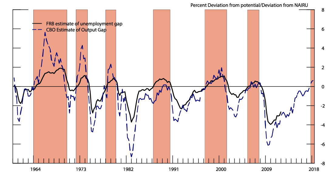
Note: The orange shading denotes periods of economic overheating. Output gap is computed as a percent deviation of real GDP from real potential GDP. Unemployment gap is computed as negative of a deviation of the unemployment rate from the FRB NAIRU estimate.
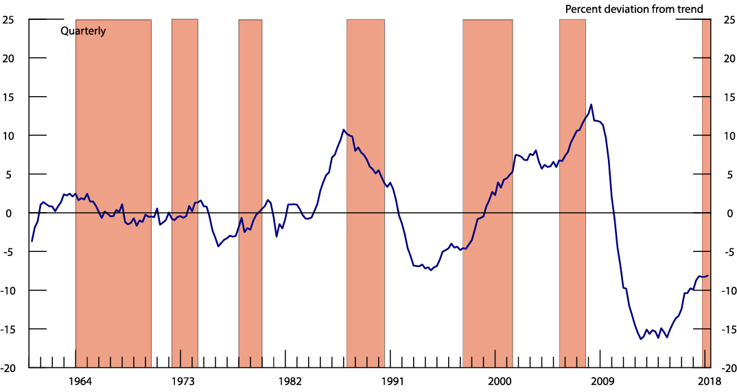
Note: The orange shading denotes periods of economic overheating. The Credit Gap is derived from a one-sided HP filter with a smoothing parameter set at 400,000.
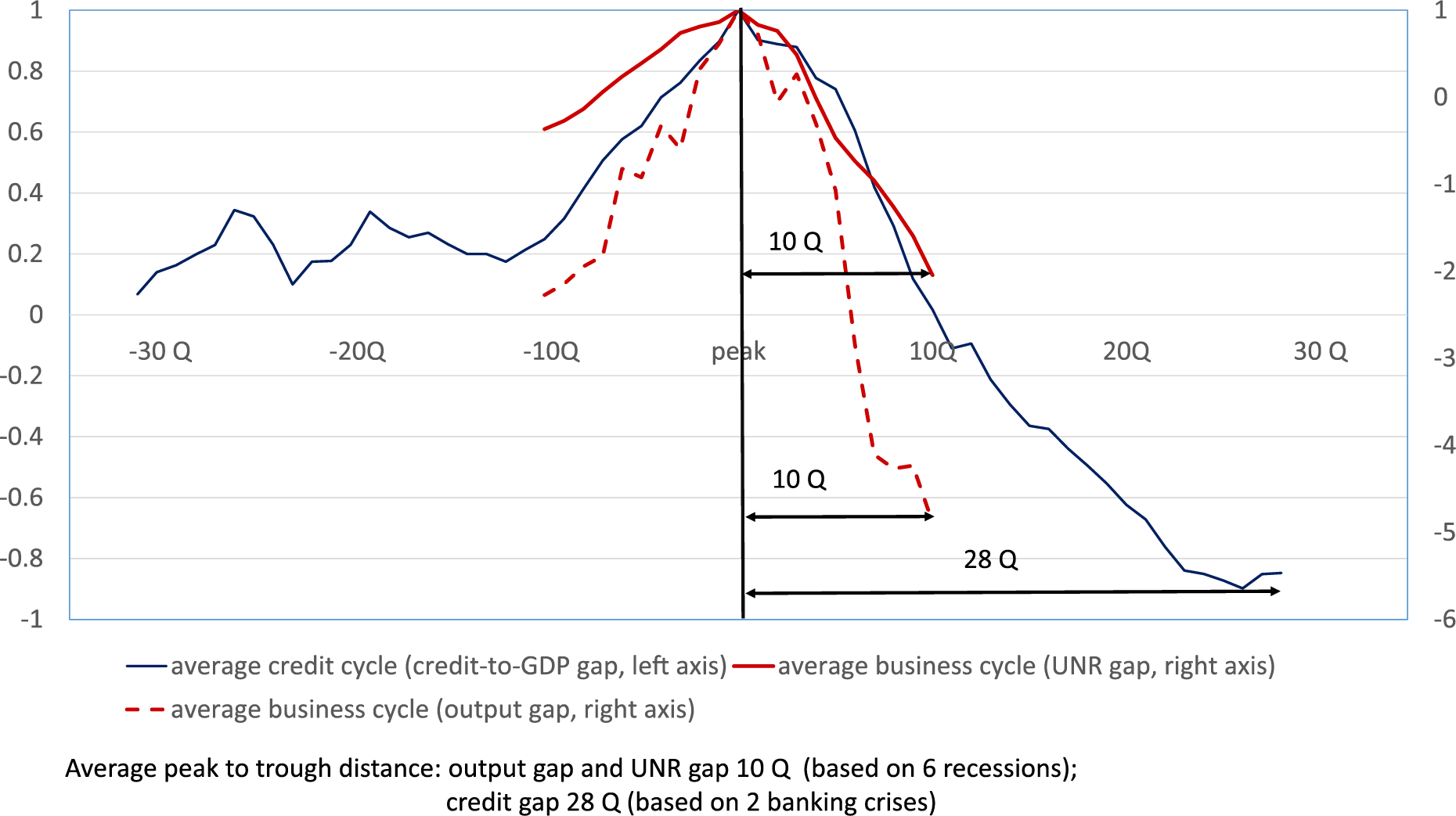
Note: The figure displays Burns-Mitchell diagrams for the credit-to-GDP gap and the measures of economic slack. The average duration of the credit cycle, measured by the typical distance from peak to trough, is shown to be 28 quarters and is substantially longer than the average duration of the business cycle (10 quarters).
Figure 3: Conditional Forecasts, Forecasts for the Credit-to-GDP Gap (one-sided) Conditional on the Output Gap
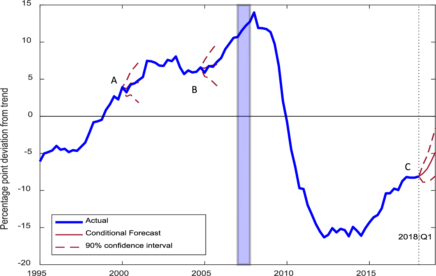
Note: The solid red lines show forecasts for the credit-to-GDP gap assuming knowledge of the path of the output gap over the following four quarters. The forecast starting in 2018:Q1 is conditional on the CBO forecasts of the output gap made in April 2018 over the following four quarters. The shaded blue area denotes the onset of the Financial Crisis.
1. We thank Alex Martin for excellent research assistance. We thank Luca Guerrieri, Michael Kiley, and Michael Palumbo for helpful comments. The note reflects the views of the authors and should not be interpreted as reflecting the views of the Board of Governors of the Federal Reserve System or anyone else associated with the Federal Reserve System. Return to text
2. Output gap is computed by the following formula: 100*(Real Gross Domestic Product – Real Potential Gross Domestic Product) / Real Potential Gross Domestic Product. Real Gross Domestic Product data from U.S. Bureau of Economic Analysis, Real Gross Domestic Product [GDPC1], retrieved from FRED, Federal Reserve Bank of St. Louis; https://fred.stlouisfed.org/series/GDPC1, July 16, 2018.; Real Potential Gross Domestic Product is from U.S. Congressional Budget Office (CBO), Real Potential Gross Domestic Product [GDPPOT], retrieved from FRED, Federal Reserve Bank of St. Louis; https://fred.stlouisfed.org/series/GDPPOT, July 16, 2018. Real potential GDP is the CBO's estimate of the output the economy would produce with a high rate of use of its capital and labor resources. The data are adjusted to remove the effects of inflation. Unemployment gap is a negative of the deviation of the unemployment rate from the Federal Reserve Board estimate of the non-accelerating inflation rate of unemployment (NAIRU), which is publicly available until the end of 2011. For further details, see https://www.philadelphiafed.org/research-and-data/real-time-center/greenbook-data/nairu-data-set. Return to text
3. A trend smoothing parameter lambda of 400.000 is used to compute the trend with the one-sided Hodrick-Prescott filter. As shown by Drehmann et al. (2010), this choice of lambda leads to the best early warning properties of the credit gap, i.e. the ability of the credit gap to signal systemic financial crises. One-sided filtering is in line with the recommendations of the Basel Committee on Banking Supervision. Return to text
4. Schularick and Taylor (2012) attribute the start of the Savings and Loans Crisis to 1984, whereas Reinhart and Rogoff (2009) report 1984-1988 as the duration of the Savings and Loans Crisis. Return to text
5. In these diagrams, an average cycle is obtained as follows. First, the peak of the cycle is isolated. Then the surrounding observations are normalized by the value of the variable at the peak. This procedure is repeated for each peak in the data span and the average across all cycles is computed. Return to text
6. Measured from trough to peak (not shown), the credit cycle is also substantially longer than the business cycle. Return to text
7. The countries in our sample include Australia, Austria, Belgium, Canada, Denmark, Finland, France, Germany, Greece, Ireland, Italy, Japan, Luxemburg, the Netherlands, Norway, Portugal, Spain, Sweden, Switzerland, and the United Kingdom. Return to text
8. The average duration of the credit cycle downturns are also downward-biased as some countries continue to experience falls in the credit-to-GDP gap up to the end of the sample period. Return to text
9. Specifically, we measure forecast accuracy with the root mean squared forecast errors (RMSFE) generated by the VARs against the RMSFE generated by an autoregressive process (AR) estimated on the variable of interest with the same number of lags as the VAR. To perform this evaluation, we split the available sample in two parts. The forecast evaluation sample spans from 1970:Q1 to 2018:Q1. The estimation strategy is recursive, starting from 1962:Q1 through the jump-off point for the forecast. For example, for a forecast starting in 1970:Q1, we estimate the VAR and AR models on samples from 1962:Q1 through 1968:Q1 for 8-step ahead forecast, through 1969:Q4 for 1-step ahead forecast. Because of data availability the VAR that includes the aggregate financial vulnerability index and the unemployment rate is evaluated on the sample 2003:Q1 to 2017:Q2, and it is estimated from 1993:Q1. This is a "pseudo out-of-sample" exercise because we disregard data revisions. As a robustness check, we estimate each of these VARs/ARs with 1 and with 4 lags of each measure. Return to text
10. We obtain similar results for the unemployment gap (not shown). Return to text
Afanasyeva, Elena, Seung Jung Lee, Michele Modugno, and Francisco Palomino (2018). "The Relationship between Macroeconomic Overheating and Financial Vulnerability: A Quantitative Exploration," FEDS Notes. Washington: Board of Governors of the Federal Reserve System, October 12, 2018, https://doi.org/10.17016/2380-7172.2254.
Disclaimer: FEDS Notes are articles in which Board staff offer their own views and present analysis on a range of topics in economics and finance. These articles are shorter and less technically oriented than FEDS Working Papers and IFDP papers.