FEDS Notes
November 12, 2020
Stuck at home? The drag of homeownership on earnings after job separation1
Eva de Francisco2, Joaquin Garcia-Cabo3, and Tyler Powell4
Introduction
This note takes a novel approach to study the question of whether housing ownership has negative effects on workers' mobility. While most of the literature has focused on studying differential migration rates between owners and renters, commonly known as "house-lock", we analyze this question from the perspective of differences in earnings.5 In particular, we compare the difference in the earnings recovery path after a job separation into unemployment or non-employment based on a worker's homeownership status at the time of the separation. This approach allows us to measure how homeowners' mobility constraints spill over into future earnings.
We use micro data from the 2004 and 2008 panels of the Survey of Income and Program Participation (SIPP). Each panel of this dataset contains several years of rich and detailed panel data for workers, including their labor histories. Moreover, by including data from both panels, spanning together the 2004-2013 time period, we can capture the stark differences in U.S. housing market conditions over time.
We show that there is a clear negative effect on earnings from owning a house in the short run. After separating from their jobs, homeowners face a slower recovery to pre-separation earnings than renters. In the long run, the impact of homeownership on earnings recovery seems to be dependent on housing market conditions. In the 2004-2008 period, the differential in earnings losses between renters and homeowners disappears after eight quarters. In the 2008-2013 period differences are persistent, even after three years, suggesting the persistent importance of the housing price collapse and slow labor market recovery during the Great Recession.
Data description
We use micro data from the Survey of Income and Program Participation (SIPP). SIPP is a longitudinal survey that collects information on household characteristics, including income, employment, and assets. It is administered by the Census Bureau. The 2004 panel contains information from 12 waves collected from February 2004 to January 2008. The 2008 SIPP panel is structured in 16 waves, with data collected between September 2008 and December 2013. Each wave contains monthly information on "core" questions (repeated in every wave) regarding the preceding four months, and "topical" questions, specific to a particular wave (or particular subset of waves). Each panel contains information from approximately 52,000 households. By using information from both panels, we analyze the role of housing on earnings recovery after job separation before and after the 2007-2009 housing bust and Great Recession.
We construct workers' labor histories using the longitudinal dimension of the panel. In particular, we define workers' employment status based on their reported status in week 2 of a given month (RWKESR2). Workers are taken to be employed in a given month if they respond "with a job" (either "working" or "not on layoff but absent without pay") in the second week of the month; unemployed if they respond "on layoff or looking for a job;" and as out of the labor force or non-employment if they are "not looking for a job and not on layoff."
Monthly earnings are constructed from information on gross pay from the primary job (TPMSUM1) for salaried workers and based on hourly rates (TPYRATE1), usual hours worked (RMHRSWK) in a week, and weeks worked in the month (RMWKWJB) for wage workers. We deflate all earnings using the consumer price index (CPI), such that all earnings are measured in 2015 dollars.6 We define (deflated) wage per hour as the ratio of monthly earnings and monthly hours worked.
ETENURE is an indicator variable that captures workers' housing status in a given month, and we restrain our analysis to homeowners and renters. We set a worker's housing status as the yearly mode of ETENURE to avoid sample inconsistencies and measurement error. Finally, we use demographics in our analysis to control for worker characteristics. We use variables for age (TAGE), sex (ESEX), and educational attainment (EEDUCATE) from the first wave to define the birth year of the worker and highest degree achieved throughout the sample period.
Empirical exercise
Sample selection
To analyze the role of housing status on labor mobility, we focus on workers who suffer a separation from their job (into unemployment or non-employment) between 2004Q4 and 2006Q2 in the 2004 wave and between 2009Q3 and 2011Q4 in the 2008 wave. We define these group of workers as the treatment group. We compare their earnings relative to a group of workers (control group) who do not separate from their jobs during that time frame.7
We record a separation in a month when an employed worker who was working and not absent from work in the previous month reports no employment. We believe that excluding workers that declare to be employed but absent without pay from this definition avoids counting temporary layoffs and furloughs, reducing respondent bias in our sample. We require workers at the time of separation to be between 30 and 55 years old, so we capture prime-age homeowners and avoid the distorting labor market decisions that occur closer to retirement.8 We further restrict workers to have at least three years of work tenure in the year when separations start and to be employed full-time. We additionally require all workers to have positive earnings in at least one year following the start of separations. We focus on workers whose homeownership status does not change between 2004-2006 and 2009-2011 for the 2004 and 2008 panels, respectively.9
Econometric model
Following Davis and von Wachter (2011), we estimate the following distributed-lag model for earnings in an unbalanced panel:
$$$$ (1) \ \ e_{it} = \alpha_i + \gamma_t + \beta X_{it} + \beta^H X_{it} I^H + \sum_{k \ge -2}^{12} {\delta_k D^k_{it}} + \sum _{k \ge -2}^{12} {\delta^H_k D^k_{it} I^H} + \varepsilon_{it} $$$$
In our baseline model, we regress quarterly earnings, for all individuals $$i$$ over time (quarter and year) $$t$$, on person fixed effects, $$\alpha$$, year fixed effects, $$\gamma$$, and a quadratic polynomial in age, $$X$$. The dummy $$I^H$$ takes value 1 if the worker is a homeowner at the time of separation, and 0 if they are a renter. Earnings losses of the treatment group are measured through the set of dummies $$D^k_{it}$$, where $$k$$ keeps track of the number of quarters before or after separation. We use information for up to 4 quarters before the separation and we mark 0 as the quarter of separation, following workers for up to 12 quarters after.10 With this specification we can compute the change in earnings $$k$$ quarters after separation by homeownership status prior to separation. Hence, $$\delta_k + \delta^H_k$$ captures the earnings losses of homeowners, and $$\delta_k$$ the earnings losses of renters, relative to similar workers who did not separate from their employers into unemployment or non-employment.11
Results
A comparison in time
By using the 2004 and the 2008 waves of SIPP, our data shows the earnings recoveries of renters and homeowners after job separations, not only during the particular circumstances that collided during the Great recession, but also during the earlier period of healthy economic growth.
Figure 1 shows the losses of earnings for homeowners and renters who were separated during the 2004 and 2008 waves of SIPP and their different recovery paths. Although it is expected that because homeowners start with higher salaries, they also suffer larger losses on average after separation, the main takeaway of Figure 1 is that for most of the first two years after a separation, homeowners' earnings recoveries lag those of renters.12
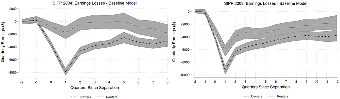
(Left Image) Source: Authors’ calculations using SIPP 2004 data (U.S. Census Bureau)
Note: Shading represents 90 percent confidence interval
(Right Image) Source: Authors’ calculations using SIPP 2008 data (U.S. Census Bureau)
Note: Shading represents 90 percent confidence interval
A potential candidate to explain this finding is the presence of a house-lock effect that can act through multiple channels. For example, social attachment to an area or school can make homeowners stay in an area in spite of worsening job prospects. Financially, home equity lines can allow homeowners to be pickier when accepting new job offers, but can also lead to human capital losses, making finding a job in the future more difficult. Moreover, homeowners may also be reluctant to incur the high transaction costs of selling a house and may restrict their job search to their current commuting zone.13 However, a clear message emerges from Figure 1: the negative friction from homeownership was present not only when house prices collapsed during the Great Recession, and financial conditions tightened significantly, but also during 2004, when these factors were not at play.
Additionally, it is evident from Figure 1 that in the 2008 panel, amid a large economic contraction, earnings losses for both homeowners and renters were larger and recoveries slower than those of similar workers in the 2004 panel. This is in line with the results of Davis and von Wachter (2011) on scarring being more severe during recessions. Interestingly, renters' losses are non-significant one year after separation in the 2004 panel, in contrast with losses of around 3,500 dollars one year after job separation in the 2008 panel. Homeowners on the other hand, suffer significant and persistent losses in both time periods, albeit larger in the 2008 panel.
Note that two years post-separation, the earnings differences between homeowners and renters in the 2004 panel are not statistically significantly different from each other. However, in the 2008 panel, shown on the right side of Figure 1, the earnings loss gap between renters and homeowners remains about 2,000 dollars, even three years after a separation, and these differences are statistically significant at the 10% level.
Figure 2 presents the results of running the same regression model characterized in (1), but with log earnings as the dependent variable. This specification only considers earnings upon reemployment and excludes observations with zero earnings. Moreover, we can easily interpret the coefficients as percentage loss relative to the control.14 The main message from Figure 1 remains, that is, renters have less persistent losses than similar homeowners when they separate from firms.
A possible takeaway from comparing Figures 1 and 2 is how different the job and housing markets where between 2004 and 2008, and how that seemed to be a key factor for unemployed workers looking for a job in the two quarters immediately following a separation.
After separating in the 2004 panel, renters who found a job up to a year and a half following the separation had no significant loss in earnings compared to similar employed renters. Meanwhile, the loss of earnings for homeowners is unequivocal, showing a similar pattern independent of the macroeconomic conditions and, once again, pointing to the existence of frictions associated with homeownership.
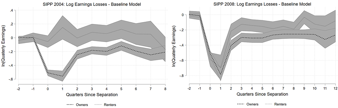
(Left Image) Source: Authors’ calculations using SIPP 2004 data (U.S. Census Bureau)
Note: Shading represents 90 percent confidence interval
(Right Image) Source: Authors’ calculations using SIPP 2008 data (U.S. Census Bureau)
Note: Shading represents 90 percent confidence interval
Contrary to the 2004 wave, for those who found a job in the first two quarters after separation in the 2008 wave, we observe smaller differences in losses, albeit large in magnitude, for owners (80%) and renters (70%), relative to their control groups. After the second quarter, as the unemployed find jobs, the recovery of renters becomes steeper, exhibiting a smaller long-run earnings scar compared to homeowners.
A deeper look at the Great Recession
The Great Recession was a time like no other, a confluence of a rapid, broad, and persistent increase in unemployment rates, mixed with a collapse in house prices following a period of unprecedented increase in homeownership, that led a lot of households into difficult financial situations.
The left panel of Figure 3 shows earning losses of separated workers obtained after running regression (1) in states with house price declines in the 25, 50, and 75 percentile of the distribution. This shows that the average earnings losses for both renters and homeowners were larger in states that had larger decreases in house prices.
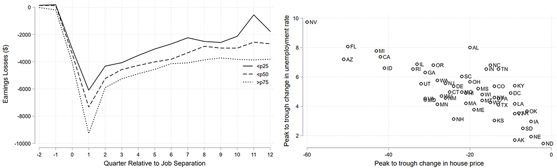
(Left Image) Source: Authors’ calculations using SIPP 2008 data (U.S. Census Bureau)
(Right Image) Source: Corelogic (2018), “House prices,” webpage, https://www.corelogic.com/downloadable-docs/corelogic-peak-totrough-final-030118.pdf Bureau of Labor Statistics
While these findings are suggestive of the role of house prices in labor reallocation, this analysis cannot lead any causal conclusions on the quantitative effect of the housing price collapse on earnings observed during the Great Recession. As shown in the right panel of Figure 3, there is a clear and strong positive correlation between increases in unemployment rates and house price declines across U.S. states.15 This justifies the need for a quantitative structural model that allows us to disentangle how the joint transmission of house price and unemployment shocks affects the real economy, and rationalize the different earnings paths after job separations between homeowners and renters.
References
Aaronson, D. and Davis, J. (2011). How much has house lock affected labor mobility and the unemployment rate? Chicago Fed Letter, Essays on Issues by The Federal Reserve Bank of Chicago, Number 290, September 2011.
Davis, M. A, Fisher, J. D. M. and Veracierto, M. (2010). The role of housing in labor reallocation. Federal Reserve Bank of Chicago, Working Paper, 2010-18.
Davis, S. J. and von Wachter, T. (2011). Recessions and the cost of job loss. Brookings Papers on Economic Activity, Fall (2), 1–72.
de Francisco, E. and Garcia-Cabo, J. (2020). Leveraged housing and job dynamics during the great recession. mimeo.
Demyanyk, Y., Hryshko, D., Luengo-Prado, M. J. and Sørensen, B. E. (2017). Moving to a job: The role of home equity, debt, and access to credit. American Economic Journal: Macroeconomics, 9 (2), 149–81.
Karahan, F. and Rhee, S. (2019). Geographic reallocation and unemployment during the great recession: The role of the housing bust. Journal of Economic Dynamics and Control, 100, 47–69.
Krolikowski, P. (2018). Choosing a control group for displaced workers. Industrial and Labor Relations Review, 71 (5), 1232–1254.
Mian, A. and Sufi, A. (2014). What explains the 2007-2009 drop in employment? Econometrica, 82 (6), 2197–2223.
Molloy, R., Smith, C. L. and Wozniak, A. (2011). Internal migration in the united states. Journal of Economic Perspectives, 25 (3), 173–196.
Schulhofer-Wohl, S. (2012). Negative equity does not reduce homeowners' mobility. Federal Reserve Bank of Minneapolis Quarterly Review, 35 (1), February 2012, 2–14.
1. We are grateful to Ben Griffy for his help and advice with SIPP database and to Shaghil Ahmed, Andrea de Michelis, and Raven Molloy for useful comments. These views are those of the authors and not necessarily those of the Board of Governors, the Federal Reserve System, the U.S. Bureau of Economic Analysis, or the U.S. Department of Commerce. Return to text
2. Bureau of Economic Analysis, [email protected] Return to text
3. Board of Governors of the Federal Reserve System, [email protected] Return to text
4. Brookings Institution, [email protected] Return to text
5. For an empirical approach see for instance Schulhofer-Wohl (2012) and Aaronson and Davis (2011). Davis et al. (2010), Karahan and Rhee (2019) and Demyanyk et al. (2017) among others present a structural approach to this question. Return to text
6. Wages come from SIPP question on hourly wages, and are corrected for topcoding comparably to the CEPR wage series. Return to text
7. Our empirical approach follows closely Krolikowski (2018) and Davis and von Wachter (2011), where we treat separations as event studies. We refer to these papers for further details. We choose the sample to have at least three quarters of pre-separation information. Return to text
8. The age restriction is applied in 2004Q4 and 2009Q3 for the control groups of workers who do not suffer a separation in each wave. Additionally, we weigh all observations in our econometric analysis using individual sample weights in 2004Q3 and 2009Q2 (before separations start for each wave). Return to text
9. In separate robustness analysis relaxing this assumption does not change our narrative. Return to text
10. For some workers the first wave interview is incomplete and we only have 3 quarters of information prior to separation. Also, the number of quarters we can observe a worker after a separation diminishes the later in the sample the separation takes place. We follow workers in the 2008 panel for up to 12 quarters, and in the 2004 panel for up to 8 quarters, since it contains fewer waves. Return to text
11. Errors are clustered at the individual level. Return to text
12. In 2004, the earnings recovery is only increasing the first 5 quarters after separation, maybe signaling a faster job finding rate of the most skilled workers (both homeowners and renters), followed by a later and poorer job match of less skilled workers (between the 5th and 8th quarter after separation). In contrast, the right panel in Figure 1 shows that the earnings recovery in the 2008 wave was increasing for all the 12 quarters for which we could follow workers. We leave the validity of this argument to explore in future research. Return to text
13. The empirical model presented here is not able to separately quantify these channels, and consequently, this question is explored in depth by using a structural model in de Francisco and Garcia-Cabo (2020). Molloy et al.(2011) investigate the role of house-lock in preventing internal migration in the United States. Return to text
14. We obtain the percentage from the approximate equivalence of ex−1=%, where x=coefficient. Return to text
15. This is not a novel observation, see for instance Mian and Sufi (2014) for further analysis. Return to text
de Francisco, Eva, Joaquin Garcia-Cabo, and Tyler Powell (2020). "Stuck at home? The drag of homeownership on earnings after job separation," FEDS Notes. Washington: Board of Governors of the Federal Reserve System, November 12, 2020, https://doi.org/10.17016/2380-7172.2802.
Disclaimer: FEDS Notes are articles in which Board staff offer their own views and present analysis on a range of topics in economics and finance. These articles are shorter and less technically oriented than FEDS Working Papers and IFDP papers.