FEDS Notes
July 08, 2021
Housing Market Tightness During COVID-19: Increased Demand or Reduced Supply?
Elliot Anenberg and Daniel Ringo1
1. Introduction
During the COVID-19 pandemic, the housing market has tightened considerably. Figure 1 shows that the months' supply of homes for sale has fallen to historically low levels. Related to this tightness, the figure also shows that house price growth has increased substantially during the pandemic. The tighter housing market could reflect increased demand (higher inflow of buyers to the market), reduced supply (lower inflow of sellers to the market), or some combination of the two. On the demand side, the pandemic forced households to spend more time at home and this increase in demand for housing services may have drawn buyers into the housing market. Lower interest rates likely also stimulated housing demand. At the same time, homeowners could be reluctant to list their home for sale during a pandemic, which could have reduced the for-sale supply. Generous mortgage forbearance programs and the foreclosure moratorium may also have reduced supply, among other factors.
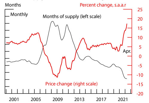
Note: Months' supply of existing homes for sale is from the National Association of Realtors, and is seasonally adjusted. Monthly house price growth is from Zillow, Inc. and is a seasonally adjusted annual rate.
In this note, we decompose the increase in housing market tightness during the pandemic into generic demand and supply factors. We find that 93 percent of the decrease in months' supply to date is driven by higher demand. Outside of a brief shock at the beginning of the pandemic, reduction of supply was a minor factor relative to increased demand in explaining the tightening of housing markets. Moreover, we show that new for-sale listings would have had to expand by 20 percent to keep months' supply and the rate of price growth at pre-pandemic levels given the pandemic-era surge in demand. This would be a very large expansion in new for-sale listings: over the last several years, total annual new listings have not changed by more than a few percent. Absent a cooling in housing demand or a substantial increase in new for-sale listings, the housing market is likely to remain very tight in the short run.
2. Model of Housing Search
To facilitate our decomposition of recent housing market tightening into demand and supply factors, we use a simple model of housing search. Supply, in this context, is defined as the monthly flow of homes coming onto the for-sale market. The total inventory of homes for sale, $$s$$, is a function of:
- this inflow of new sellers, $$n_s$$;
- the rate at which homes are sold, $$q$$; and,
- the rate at which unsold homes are withdrawn from the market, $$w$$.
An accounting identity in which the values of these inputs in month $$t$$ determines the housing stock for sale in the beginning on month $$t+1$$ is:
$$ (1) \ \ \ \ \ s_{t+1}= s_t - s_t (q_t+(1 -q_t)w_t) + (1-w_t)n_{st} $$
All of the inputs in equation 1 are directly observable or calculable from home listings data. Demand is defined as the flow of prospective buyers that enter the market to find a home to purchase. Similarly to the supply of homes for sale, there exists some stock of currently-searching buyers, $$b$$, that is replenished by this inflow, and depleted as buyers purchase a home and exit the market, or become discouraged and drop out without purchasing. No demand-side equivalent of the home listings data exists, however, so these stocks and flows remain unobservable to us. We can think of them as evolving equivalently to the supply side:
$$ (2) \ \ \ \ \ b_{t+1}=b_t-s_t q_t+n_{bt} $$
Where $$n_{bt}$$ represents the net inflow of new buyers and outflow of discouraged buyers.
Supply and demand interact via the search and matching process, which we model as an urn-ball function:
$$ (3) \ \ \ \ \ q_t=1-exp \left(-A \frac{b_t}{s_t} \right) $$
The rate of home sales, $$q$$, is determined by the market tightness (the ratio of $$b$$ to $$s$$) and a technology parameter $$A$$ that determines the efficiency of the matching function. The more interested buyers for each house there are in the market, the faster that house is likely to sell, and so $$q$$ is an increasing function of market tightness. From equation 1, a high enough $$q$$ may cause the stock of listings $$s$$ to diminish even in the presence of a high inflow of new supply, $$n_s$$. Therefore, a reduced number of listed homes for sale could be caused by higher demand (an increase in $$n_b$$ driving up $$b$$), lower supply (a reduction in $$n_s$$ reducing $$s$$), or both.2
3. Estimation
To impute the relative influence of supply and demand on recent market tightening, we first need to observe the recent histories of $$n_b$$ and $$n_s$$. We use home listings data provided by Redfin, a national real estate brokerage, to observe $$n_s$$.3 These data cover a consistent sub-set of U.S. real estate markets at a monthly frequency beginning in 2017. They include the number of new listings, withdrawals, sales, and active inventory. The net inflow of buyers, $$n_b$$, is unobserved, but can be backed out using the structure of the model described above. The solid line of Figure 2 shows the time series of $$s$$, the inventory of active listings from Redfin. Given this path for $$s_t$$ and the path for $$q_t$$ calculated from the data (shown in the black line of Figure 4), a path for $$A \cdot b_t$$ can be computed by inverting equation 3. We calibrate $$A$$ = 0.48 using Redfin data on the average sale hazard in 2019 and survey data from the National Association of Realtors (NAR) on average search time for buyers in 2019, leaving us with an estimated path for $$b_t$$.4
We plot the estimated path of $$b_t$$ as a dashed line in Figure 2. While the inventory of homes for sale has greatly diminished, the estimated population of buyers searching for a home has increased. Given this path for $$b_t$$, $$n_{bt}$$ can be backed out using equation (2). This estimated monthly inflow of new buyers is shown in Figure 3, along with observed monthly new listings, $$n_S$$. Both series are shown as changes relative to 2-years previously, to clear out seasonality.
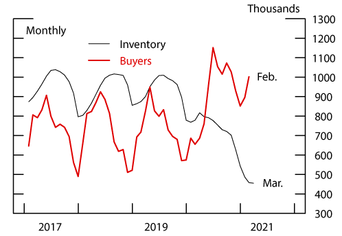
Note: Active listings inventory are data from Redfin. Stock of active buyers is estimated using the housing search model.
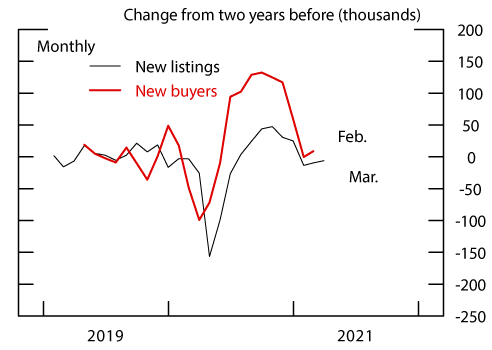
Note: New listings are data from Redfin. New buyers are the 3-month moving average of the net inflow of new buyers estimated using the housing search model.
4. Counterfactuals
We decompose the change in market tightness since March 2020 into supply and demand factors by running two counterfactual scenarios in which only one of supply or demand is allowed to follow its pandemic-era path. In the first scenario, we fix $$n_{bt}$$ at the level estimated during the equivalent calendar month in the year before the pandemic, while $$n_{st}$$ follows the observed path in the data. In the second scenario, we use the estimated path of $$n_{bt}$$ during the pandemic, while fixing $$n_{st}$$ at the levels observed in the equivalent calendar month in the year before the pandemic. Starting from the existing inventory of homes for sale (and estimated population of actively searching buyers) in February 2020, we simulate forward the paths of $$s_t$$ and $$b_t$$ under these two counterfactual scenarios. As $$s_t$$ and $$b_t$$ change, the rate of sale changes too according to equation 3.
We plot the rate of sale ($$q_t$$) implied by these scenarios, as well as the true values, in Figure 4. The scenario in which supply is unchanged but the demand for homes follows its (estimated) true path explains much more of the realized market tightening than the scenario in which demand is unchanged but supply is allowed to follow its observed path. Changes to demand alone explain 88% of the increase in q and 93% of the decrease in months' supply (defined as $$1/q$$) between March 2020 and March 2021. We conclude that, outside of a brief shock at the beginning of the pandemic, reduction of supply was a minor factor relative to increased demand in explaining the tightening of housing markets. We run a third set of counterfactual simulations, in which demand ($$n_{bt}$$) is set at its actual estimated levels, but supply ($$n_{st}$$) is set at some multiplier, $$x$$, of the equivalent calendar month in the year before the pandemic. We find that a value of $$x$$ = 1.2 or greater is necessary to bring the counterfactual $$q$$ back to its pre-pandemic level by March 2021. This means that a 20% increase in the monthly number of homes coming on to the market would have been necessary to keep up with the pandemic-era surge in demand.
5. Implications for House Prices
How much of the rise in house prices during the pandemic can we attribute to a demand-driven increase in market tightness? To get a sense of its contribution, we first estimate a simple model of house price growth as
$$ (4) \ \ \ \ \ \Delta log(p_t)= \beta_0 + \beta_1 \Delta log(q_{t-1}) + \varepsilon_t $$
Where $$ \Delta log(p_t) $$ is the monthly log change in the real median sale price from the Redfin data. Estimating equation 4 using OLS and excluding the pandemic period from the estimation sample, we find a positive and statistically significant estimate for $$\beta_1$$. The R-squared of the regression is 0.44, meaning that the change in sale hazard alone can explain almost half of the variation in the change in house prices over our sample period.
For each of the two counterfactual paths of $$q_t$$ shown in Figure 4, we compute an estimate for $$log(p)$$ using the same estimated parameters and residuals from equation 4, but feeding in our counterfactual sale hazards. We set the residuals, $$\hat{\varepsilon}_t$$, equal to year-earlier levels for months after March 2020. As a result, only demand or supply changes in each counterfactual relative to the pre-pandemic period. Figure 5 shows the results of the two counterfactual price series compared to the actual price series. At the beginning of the pandemic, reduced supply could explain the rise in house prices. However, as the pandemic continued, the role of supply decreased and increased demand drove house prices higher. As of March 2021, we find that almost all of the increase in house prices during the pandemic can be attributed to increased demand.
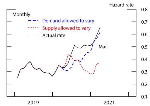
Note: Actual monthly sale hazard rate is computed from Redfin data.
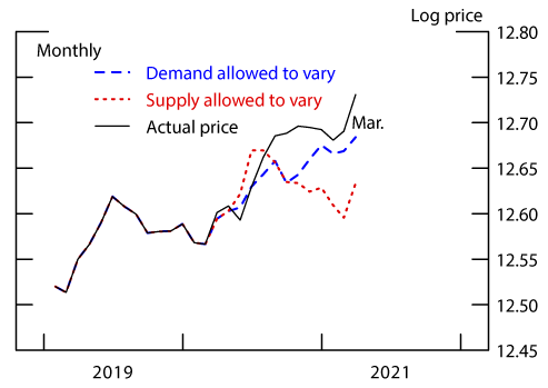
Note: Actual log median real sale price is from Redfin.
6. Discussion
This analysis indicates that the housing market has tightened primarily because of a surge in demand. Consequently, the relaxation of any pandemic-caused supply-side constraints will likely do little to cool the market. New demand has exceeded even pre-pandemic levels of supply, and the gap is too large to be realistically filled by new construction in the short term. The lack of gains in new listings might be surprising given that many homebuyers are owner-occupants who would be expected to sell their current home when purchasing a new one. However, the pandemic has seen an increase in second-home buying, and these purchases would not generate new subsequent listings.5 Another contributing factor could be that, in tight markets, homeowners attempt to buy their next home before putting their current home on the market, as they can be confident of finding a buyer quickly. Additional research is needed to understand the factors that caused a surge in new buyers without a corresponding increase in new listings.
1. The analysis and conclusions set forth are those of the authors and do not indicate concurrence by other members of the research staff or the Board of Governors. Return to text
2. An increase in the listing withdrawal hazard, $$w$$, would have an equivalent effect on inventories and tightness as a reduction in $$n_s$$. However, our data indicate little change in the withdrawal rate over our sample period. Return to text
3. https://www.redfin.com Return to text
4. The ratio of the sale hazard to the purchase hazard implied by the NAR data gives an estimate of the market tightness, which we can plug into equation 3 to solve for $$A$$. Social distancing may have disrupted some aspects of home search, particularly earlier in the pandemic, leading to less efficient search (i.e. a lower value of $$A$$). A decline in the efficiency of the matching function during the pandemic would imply an even greater surge in demand than we estimate to rationalize observed market tightness. In general, however, the results in this note are qualitatively similar even if much higher or lower values of $$A$$ are used. We also find similar or stronger results using a Cobb-Douglas function (instead of the urn-ball described in equation 3) under a wide range of calibrations. Return to text
5. The market share of first-time buyers (who also do not produce new listings) has been little changed. Return to text
Anenberg, Elliot, and Daniel Ringo (2021). "Housing Market Tightness During COVID-19: Increased Demand or Reduced Supply?," FEDS Notes. Washington: Board of Governors of the Federal Reserve System, July 08, 2021, https://doi.org/10.17016/2380-7172.2942.
Disclaimer: FEDS Notes are articles in which Board staff offer their own views and present analysis on a range of topics in economics and finance. These articles are shorter and less technically oriented than FEDS Working Papers and IFDP papers.