FEDS Notes
June 19, 2020
Measuring the Natural Rate of Interest: The Role of Inflation Expectations
David Lopez-Salido, Gerardo Sanz-Maldonado, Carly Schippits, and Min Wei
Introduction and Motivation
The "natural" or equilibrium real rate of interest is an important concept in macroeconomics. On the one hand, the natural (real) rate provides a description of the real interest rate path consistent with the eventual full capacity of utilization of available resources in the context of low and stable inflation. On the other hand, the natural rate is also an important "reference" for monetary policy, since it is a key determinant of a variety of simple policy rules that are often used to characterize monetary policy.
In an important contribution to the literature, Laubach and Williams (2003, henceforth LW) and Holston, Laubach, and Williams (2017, henceforth HLW) use a simple aggregate demand and aggregate supply model of the economy to estimate the natural rate of interest in the U.S. over the past 60 years.
In this note, we keep the LW and HLW framework, but discuss how the results vary when we make a small change to the estimation strategy. In particular, we study how the level and variability of the estimated natural rate of interest depend on variables used to approximate the underlying inflation expectations. This exercise is motivated by two observations: first, short-run inflation expectations directly determine the ex-ante short-run real rate; second, increased anchoring of longer-run inflation expectations is an important feature over our sample period (1961 to 2019), and it is important to account for this trend when estimating the Phillips curve.
Our emphasis on inflation expectations is in line with recent efforts to understand inflation dynamics, in particular the theoretical and empirical work on to what extent backward-looking expectations—i.e. those giving a prominent role to past inflation—instead of forward-looking expectations—proxied here by survey forecasts—are useful components of empirical models of inflation.1 It is notable that this discussion has not played much of a role in the empirical analysis of the determinants of the equilibrium real rate. Instead, the discussion has centered on the sensitivity of the estimates to parameter uncertainty and alternative specifications (e.g., Lewis and Vazquez-Grande, 2019) or the role of global factors (Kiley, 2019).
We have two main findings. First, incorporating information from long-run survey forecasts of inflation leads to a sharper decline in the estimated natural rate of interest since the early 2000s, with the estimate for 2019Q4 still below zero. The lower level of estimates comes from the fact that long-run survey inflation forecasts stayed above realized inflation for much of this period, translating into a lower output gap and hence a lower $$r^*_t$$ than those implied by the backward-looking measure used in HLW. Second, incorporating information from short-run survey forecasts helps reduce the uncertainty surrounding the estimates of $$r^*_t$$, as exemplified by the narrower confidence bands, while having little effect on the level of estimates.
An Abridged Presentation of the HLW Model
Let $$\tilde{y_t} = y_t - y^*_t$$ and $$\tilde{r_t} = r_t – r^*_t$$ denote the deviations of log real GDP, $$y_t$$, and the real short rate, $$r_t$$, from their respective natural or equilibrium levels, $$y^*_t$$ and $$r^*_t$$. In the LW-HLW model, an investment-saving (IS) or aggregate demand equation governs the evolution of the output gap, $$\tilde{y_t}$$,
$$ (1) \ \ \ \ \ \ \ \tilde{y}_t = a_{y,1}\tilde{y}_{t-1} + a_{y,2}\tilde{y}_{t-2} + \frac{a_r}{2} \sum_{j=1}^2 \tilde{r}_{t-j} + \varepsilon_{\tilde{y},t}, $$
where potential output, $$y^*_t$$, is assumed to follow a random walk with a stochastic drift $$g_t$$,
$$ (2) \ \ \ \ \ \ \ y^*_t = y^*_{t-1} + g_{t-1} + \varepsilon_{y^*,t}, $$
while a Phillips curve or aggregate supply equation governs the evolution of inflation, $$\pi_t$$,
$$ (3) \ \ \ \ \ \ \ \pi_t = b_{\pi}\pi_{t-1} + (1-b_{\pi})\pi^*_t + b_y\tilde{y}_{t-1} + \varepsilon_{\pi,t}, $$
where $$\pi^*_t$$ is the trend inflation. LW and HLW specify the natural rate, $$r^*_t$$, as the sum of two components, the trend growth rate of potential output, $$g_t$$, and other determinants of the natural rate, $$z_t$$, with both $$g_t$$ and $$z_t$$ assumed to follow random walks:
$$ (4) \ \ \ \ \ \ \ r^*_t = g_t + z_t $$; $$g_t = g_{t-1} + \varepsilon_{g,t} $$; $$z_t = z_{t-1} + \varepsilon_{z,t} $$.
The model is closed by noting that the nominal short rate, $$i_t$$, is linked to the real short rate and expected inflation, $$E_t\pi_{t+1}$$, through the Fisher Equation:
$$ (5) \ \ \ \ \ \ \ i_t = r_t + E_t\pi_{t+1} $$.
The HLW model can be estimated using either PCE inflation—as done in their papers—or CPI inflation. To see whether the model might be sensitive to using these two measures of inflation, Panel A of Figure 1 plots one-quarter core PCE and core CPI inflation over the sample period of 1960Q1-2019Q4. The two measures follow a broadly similar contour, rising gradually through the 1960s and 1970s, peaking in the mid to late 1980s, gradually declining over the next twenty years, and fluctuating around 2 percent since the mid-1990s. There are some disparities between the two series over certain periods. For example, CPI inflation spiked more than PCE inflation in response to the second oil shock in 1979 and lied above PCE inflation over the entire 1990s. However, the differences are relatively small compared to the range of their values and have shrunk further since 2000.
Panel B plots the resulting estimates of $$r^*_t$$ from the HLW model using core PCE and core CPI inflation, respectively.2 Despite some small differences in particular time periods, the variations of the two series are quite similar over the entire sample.3
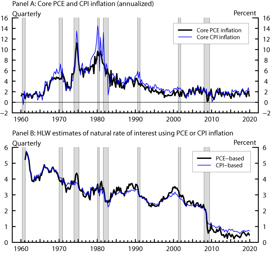
In addition, Table 1 shows that the choice of the inflation measure leads to only small differences in the parameter estimates of the model. The two sets of estimates imply similar degrees of persistence for inflation and output ($$a_y$$ and $$b_{\pi}$$). The most noticeable difference is in the slope of the inflation equation ($$b_y$$). Using core CPI inflation identifies a steeper Phillips curve, with an estimated pass-through from changes in the output gap to inflation more than double that using core PCE inflation. Finally, the CPI-based estimation generates a slightly lower elasticity of the output gap to changes in the real interest rate gap ($$a_r$$).
Table 1: Parameter estimates using PCE or CPI inflation
| PCE-based | CPI-based | |
|---|---|---|
| Sample | 1961:Q1-2019:Q4 | 1961:Q1-2019:Q4 |
| $$\sum a_y$$ | 0.941 | 0.929 |
| $$a_{y,1}$$ | 1.540 | 1.624 |
| $$a_{y,2}$$ | -0.599 | -0.695 |
| $$a_r$$ | -0.068 | -0.043 |
| $$b_{\pi}$$ | 0.671 | 0.604 |
| $$b_y$$ | 0.079 | 0.197 |
| $$\sigma_{\tilde{y}}$$ | 0.334 | 0.328 |
| $$\sigma_{\pi}$$ | 0.786 | 1.166 |
| $$\sigma_{y^*}$$ | 0.574 | 0.585 |
| $$\sigma_g$$ | 0.031 | 0.023 |
| $$\sigma_z$$ | -0.174 | -0.112 |
| $$\sigma_{r^*} = \sqrt{\sigma_g^2 + \sigma_z^2}$$ | 0.177 | 0.115 |
| $$\lambda_g = \frac{\sigma_g}{\sigma_{y^*}}$$ | 0.053 | 0.040 |
| $$\lambda_z = \frac{a_r \sigma_z}{\sigma_{\tilde{y}}}$$ | 0.035 | 0.015 |
The evidence so far suggests that replacing core PCE inflation by core CPI inflation in the original HLW model does not significantly affect their estimates. With this in mind and for reasons that will become clear soon, in the rest of this note we will focus on model estimates based on CPI inflation.
HLW and Inflation Expectations
Two inflation expectation measures play an important role in the HLW model. First, the trend inflation term, $$\pi^*_t$$, appearing in the Phillips curve equation (3), affects our inference about the unobserved output gap based on realized inflation. Similarly, in the IS equation (1), the 1-quarter ahead expected inflation, $$E_t \pi_{t+1}$$, by affecting the measurement of the ex-ante real rate $$r_t$$ according to Equation (5), influences the inference regarding the dynamics of the real rate gap for a given history of output gap and nominal short rates. These observations suggest that model estimates of $$r^*_t$$ may be crucially influenced by how we measure or proxy those two inflation expectations terms.
In their implementation, HLW use current and past inflation to proxy for trend inflation and short-run inflation expectations. In particular, they measure trend inflation using average core inflation over the past two through four quarters ($$\frac{1}{3}\sum_{i=2}^4 \pi_{t-i}$$), and measure the one-quarter ahead inflation expectations using average core inflation over the past four quarters ($$\frac{1}{4}\sum_{i=0}^3 \pi_{t-i}$$). In this note, we investigate how the results change when we replace those backward-looking proxies with more forward-looking survey inflation forecasts.
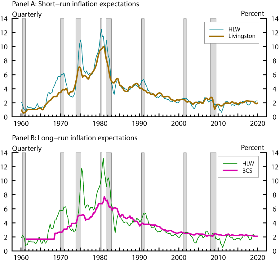
In particular, we use the 1-year ahead median CPI inflation forecast from the Livingston survey starting in 1960Q1, and the 10-year ahead CPI inflation forecast from Consensus Economics, extended by Blanchard, Cerutti, and Summers (2015, henceforth BCS) back to 1961Q2. Survey forecasts for PCE inflation only became available very recently, starting in 2007 from the Survey of Professional Forecasters and in 2014 from Blue Chip Economic Indicators. The longer history of survey forecasts of CPI inflation is the reason we focus on this measure.4
Figure 2 compares the two survey inflation forecasts with the corresponding backward-looking inflation expectation measures used by HLW. Although the survey measures and the HLW measures generally move in tandem, there are high-frequency as well as persistent differences. In particular, the survey measures tend to run below the HLW measures before 1980 and above since. The differences are more pronounced for the pre-1980 sample and for longer-run expectations. Finally, the longer-run survey inflation forecast is less volatile than the shorter-run counterpart, and exhibits a remarkable stability around 2 percent during the last twenty years.
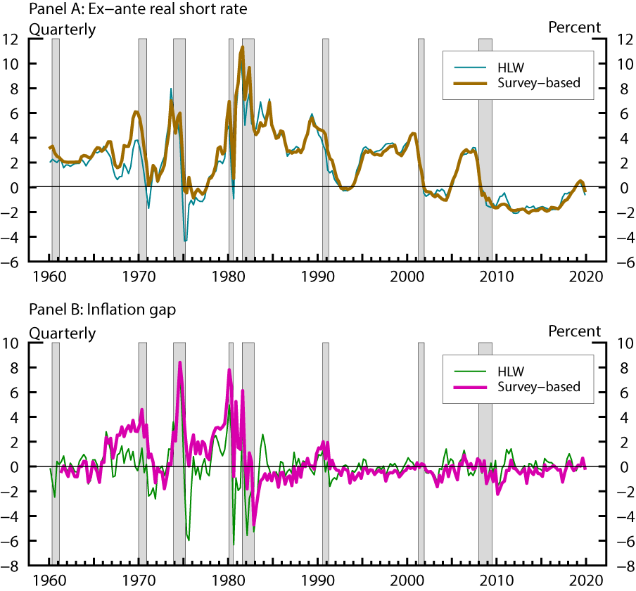
The top and bottom panels of Figure 3 plot two key variables—the ex-ante real short rate and the inflation gap—that enter into the HLW model and are directly affected by the proxies used to measure inflation expectations. The ex-ante real short rate is calculated by subtracting either measure of the short-run inflation expectations displayed in the top panel of Figure 2 from the observed nominal short rate. The survey-based real short rate is mostly above the HLW measure and is less volatile in the first half of the sample. The volatilities of both measures are considerably reduced during the so-called "Great Moderation" period (i.e. from the late 80s or early 90s onward). During this period, the survey-based real short rate tends to slightly undershoot the HLW measure. Overall, both measures are largely synchronized and have a high correlation of about 0.95 over the full sample.
The two inflation gap measures, shown in the bottom panel of Figure 3, are constructed as the difference between observed core CPI inflation and either measure of trend inflation, shown in the bottom panel of Figure 2. The volatilities of, and the correlation between, the two measures changed notably around the late 80s and early 90s. The first part of the sample witnessed substantial disparities between the two inflation gap measures. The survey-based measure was positive late in the 60s and spiked twice in the 70s, as actual price increases outpaced survey inflation expectations. In contrast, the HLW measure took both positive and negative values during the 1970s, falling sharply in the aftermath of the first oil shock and staying systematically below the survey-based measure. Subsequently, the Great Moderation period—especially if considered as having started in the early 90s—muted the volatility of both measures. The two measures became highly correlated, albeit the survey-based measure tends to run slightly below the HLW measure—particularly during the aftermath of the global financial crisis, when inflation systematically undershot the FOMC's 2 percent objective but survey inflation expectations held surprisingly stable. The correlation between the two inflation gap series, at about 0.6 over the full sample, is much lower than that of the ex-ante real short rates.
Results and Discussion
We consider four specifications of the model, depending on whether the two inflation expectation terms are measured using surveys ("Liv" or "BCS") or using past inflation as in HLW ("HLW"). We use a naming convention where the first term represents the long-run measure, whereas the second term represents the short-run measure. For example, the specification "HLW-HLW" refers to the original HLW model using past inflation to measure both short- and long-run inflation expectations, whereas the specification "BCS-Liv" refers to a model where the long-run measure is from BCS while the short-run measure is from the Livingston survey.
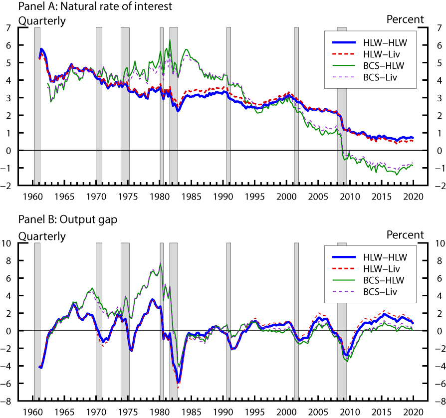
Figure 4 plots estimates of the natural rate in Panel A and the output gap in Panel B for all four specifications. Our main finding is that estimates of the natural rate and output gap in the HLW framework are materially affected by assumptions about long-run inflation expectations, while measuring short-run inflation expectations with surveys rather than past inflation appears to make a smaller difference. This is consistent with Figure 2, which shows that the backward-looking measure used by HLW appears to be a reasonable proxy for the short-run survey forecast of inflation, but works less well at longer horizons.
More specifically, regardless of how one measures short-run inflation expectations, replacing the HLW measure of long-run inflation expectations with BCS inflation forecasts leads to higher estimates of the natural rate from 1970 to 1995 but lower estimates over the past 25 years, resulting in a much steeper downward trend in the estimated natural rate from the 1980s through 2010. A similar but less dramatic change is observed for the output gap estimates. Part of the reason for these differences were already apparent from Figures 2 and 3. In particular, compared with the HLW measure, the lower level of long-run survey inflation forecasts in the earlier half of the sample, Figure 2, results in a higher inflation gap, Figure 3, which translates into a higher output gap through Equation (3) and in turn a higher natural real rate of interest through Equation (1). The opposite is true for the more recent sample.
Table 2. Parameter estimates across specifications
| HLW-HLW | HLW-Liv | BCS-HLW | BCS-Liv | |
|---|---|---|---|---|
| Sample | 1961:Q1-2019:Q4 | 1961:Q1-2019:Q4 | 1962:Q2-2019:Q4 | 1962:Q2-2019:Q4 |
| $$\sum a_y$$ | 0.929 | 0.921 | 0.957 | 0.960 |
| $$a_{y,1}$$ | 1.624 | 1.510 | 1.716 | 1.551 |
| $$a_{y,2}$$ | -0.695 | -0.590 | -0.758 | -0.591 |
| $$a_r$$ | -0.043 | -0.065 | -0.049 | -0.073 |
| $$b_{\pi}$$ | 0.604 | 0.606 | 0.485 | 0.483 |
| $$b_y$$ | 0.197 | 0.192 | 0.257 | 0.258 |
| $$\sigma_{\tilde{y}}$$ | 0.328 | 0.350 | 0.265 | 0.332 |
| $$\sigma_{\pi}$$ | 1.166 | 1.168 | 1.074 | 1.075 |
| $$\sigma_{y^*}$$ | 0.585 | 0.575 | 0.602 | 0.576 |
| $$\sigma_g$$ | 0.023 | 0.023 | 0.039 | 0.037 |
| $$\sigma_z$$ | -0.112 | -0.105 | -0.244 | -0.184 |
| $$\sigma_{r^*} = \sqrt{\sigma_g^2 + \sigma_z^2}$$ | 0.115 | 0.248 | 0.247 | 0.188 |
| $$\lambda_g = \frac{\sigma_g}{\sigma_{y^*}}$$ | 0.040 | 0.040 | 0.064 | 0.064 |
| $$\lambda_z = \frac{a_r \sigma_z}{\sigma_{\tilde{y}}}$$ | 0.015 | 0.019 | 0.045 | 0.040 |
| S.E. (sample average) | ||||
| $$r^*_t$$ | 1.134 | 0.916 | 1.246 | 1.007 |
| $$y^*_t$$ | 1.137 | 1.141 | 1.159 | 1.138 |
| Average $$r^*_t$$ | ||||
| 2015-2019 | 0.699 | 0.529 | -1.076 | -0.898 |
Table 2 compares the parameter estimates across specifications. We first note that the parameter estimates are similar across the HLW-HLW and HLW-Liv models, again reflecting the small difference in the two short-run inflation expectations measures.
For specifications that use the long-run BCS inflation forecasts, we see greater differences in parameter estimates, compared to the HLW model. In particular, the sensitivity of the output gap to the interest rate becomes greater (i.e. $$a_r$$ is more negative), inflation becomes slightly less persistent (i.e. $$b_{\pi}$$ is smaller), and the Phillips curve becomes slightly steeper (i.e. $$b_y$$ is larger), while the trend growth rate of potential output becomes relatively less important for determining the natural rate (as seen by a smaller rise in $$\lambda_g$$ relative to $$\lambda_z$$ when compared with the baseline HLW model).
Most notably, for both specifications using the long-run BCS forecasts, the average estimate of the natural rate over the past five years, reported in the last row of Table 2, is close to -1 percent, much lower than that implied by the HLW model. We caution though that this result does not necessarily imply that the true natural rate is so negative, as other considerations could have an offsetting effect on the estimate.5
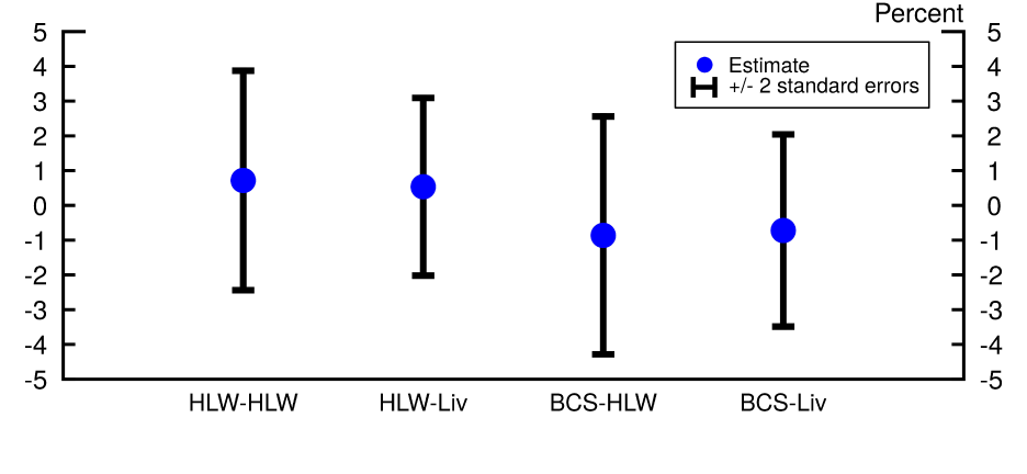
Lastly, we examine how bringing in information from survey forecasts affects the uncertainty surrounding the natural rate estimates. Figure 5 plots the natural rate estimates for 2019:Q4 together with two-standard-deviation bands across the four model specifications.6,7 Using a survey-based measure of short-run inflation expectations appears to narrow the width of the confidence interval slightly, but it does not dramatically alter the level of the natural rate estimate, compared to models using the HLW measure. This reduction in uncertainty could be explained by the fact that the Livingston inflation forecast is less volatile than the HLW measure, as can be seen in Panel A of Figure 2. We note that most of the reduction in uncertainty comes from reduced uncertainty about the value of $$z_t$$ (which captures shocks to aggregate demand) rather than about the value of $$g_t$$ (which is the growth rate of potential output).
By contrast, using survey-based measures of long-run inflation expectations shifts the entire confidence interval down. According to both BCS models, there is essentially no chance that the natural rate exceeded 2.5 percent in 2019:Q4, while according to the BCS-Liv specification, there is no chance that the natural rate exceeded 2 percent. This stands in sharp contrast to the HLW model, which places about 13 percent probability on the natural rate exceeding 2.5 percent in that quarter.
References
Blanchard, Olivier and Eugenio Cerutti and Lawrence Summers, 2015. "Inflation and Activity – Two Explorations and their Monetary Policy Implications," NBER Working Papers 21726.
Bernanke, Ben, 2007. "Inflation Expectations and Inflation Forecasting," Speech at the Monetary Economics Workshop of the National Bureau of Economic Research Summer Institute, Cambridge, Massachusetts, July 10.
Coibion, Olivier, and Yuriy Gorodnichenko, 2015, "Is the Phillips curve Alive and Well After All? Inflation Expectations and the Missing Disinflation," American Economic Journal: Macroeconomics 7, 197-232.
Holston, Kathryn, and Thomas Laubach and John C. Williams, 2017, "Measuring the Natural Rate of Interest: International Trends and Determinants," Journal of International Economics 108, supplement 1 (May): S39–S75.
Hamilton, James D., 1986. "A standard error for the estimated state vector of a state-space model," Journal of Econometrics 33(3), 387-397.
Kiley, Michael T., 2019, "The Global Equilibrium Real Interest Rate: Concepts, Estimates, and Challenges," Finance and Economics Discussion Series 2019-076. Washington: Board of Governors of the Federal Reserve System,
Laubach, Thomas, and John C. Williams, 2003. "Measuring the Natural Rate of Interest," Review of Economics and Statistics 85, no.4 (November): 1063-70.
Lewis, Kurt F., and Francisco Vazquez‐Grande, 2019, "Measuring the natural rate of interest: A note on transitory shocks," Journal of Applied Econometrics, Vol. 34, Issue 3, pp. 425-436.
Mishkin, Frederic S., 2007, "Inflation Dynamics," National Bureau of Economic Research Working Paper no. 13147, June.
1. See, for instance, Mishkin (2007) and Bernanke (2007), and recently Coibion and Gorodnichenko (2015) and the references therein. Return to text
2. We follow the estimation procedure of Holston, Laubach, and Williams (2017) using the replication code the authors kindly made available at https://www.newyorkfed.org/research/policy/rstar. Return to text
3. For the perceptive reader, we note that the average difference between the two $$r^*_t$$ estimates is about 25 basis points over the last ten years. Return to text
4. We also experimented with estimating the model using PCE inflation forecasts from the Survey of Professional Forecasters and Blue Chip Economic Indicators, extending the series back to 1960Q1 using CPI inflation expectations while taking into account the difference between observed core CPI and core PCE inflation. The conclusions are similar. Return to text
5. For example, Lewis and Vazquez-Grande (2019) show that allowing transitory rather than permanent shocks to the non-growth part of the natural rate, $$z_t$$, leads to a higher estimate of the natural rate. Return to text
6. Standard errors are computed using Hamilton's (1986) Monte Carlo procedure that accounts for both filtering and parameter uncertainty. See HLW's footnote 7 for more details. Return to text
7. The patterns seen in this chart extend to the rest of the sample period. Return to text
Lopez-Salido, David, Gerardo Sanz-Maldonado, Carly Schippits, and Min Wei (2020). "Measuring the Natural Rate of Interest: The Role of Inflation Expectations," FEDS Notes. Washington: Board of Governors of the Federal Reserve System, June 19, 2020, https://doi.org/10.17016/2380-7172.2593.
Disclaimer: FEDS Notes are articles in which Board staff offer their own views and present analysis on a range of topics in economics and finance. These articles are shorter and less technically oriented than FEDS Working Papers and IFDP papers.