FEDS Notes
September 18, 2020
Underlying Inflation: Its Measurement and Significance
Underlying inflation is the rate of inflation that would be expected to eventually prevail in the absence of economic slack, supply shocks, idiosyncratic relative price changes, or other disturbances.2 Underlying inflation is a useful benchmark for monetary policy in that it provides an idea of the rate of price change that would be expected to obtain under "normal" circumstances in an economy where the level of resource utilization is putting neither upward nor downward pressure on inflation. In addition, examination of the behavior of measures of underlying inflation over time can highlight interesting and potentially policy-relevant features of the inflation process.
Because underlying inflation is defined in terms of a state of the economy that is unlikely to ever be exactly realized, it cannot be directly observed; rather, it must be inferred from the behavior of actual inflation, either in a univariate context or with additional reference to the behavior of inflation's other determinants. In this note, I describe and assess several empirical approaches that one might use in order to generate estimates of underlying inflation. I present results from each approach, and discuss some possible implications of these results for monetary policy.
In what follows, I define inflation as the annualized log difference of the price index for personal consumption expenditures (PCE) excluding food and energy, also known as "core" PCE inflation.3 This focus on core PCE inflation is informed by two considerations. First, using the PCE price index as a starting point (rather than, say, the CPI or the GDP price index) reflects the fact that the Federal Reserve's longer-run inflation goal is defined in terms of this measure. Second, removing food and energy prices omits a source of difficult-to-model variability in overall inflation; doing so makes it easier to implement multivariate estimation approaches, and should also help to yield better estimates from univariate models.4
Univariate estimates of underlying inflation
In a 2007 paper, Stock and Watson proposed the following empirical characterization of inflation dynamics:
$$ \ \ \ \ \ \ \ \ \ \ \pi_t = \pi^{\ast}_t + \varepsilon_t $$
(1)
$$ \ \ \ \ \ \ \ \ \ \ \pi^{\ast}_t = \pi^{\ast}_{t-1} + \eta_t , $$
where $$\pi$$ is actual inflation, $$\pi^{\ast}$$ is trend inflation, and $$\varepsilon$$ and $$\eta$$ are zero-mean, serially uncorrelated innovation terms (shocks) whose variances are allowed to change randomly over time (a property known as "stochastic volatility").
In this framework, trend inflation can move around from period to period.5 At any given time $$t$$, however, the value of the trend that we expect to prevail now and at all future dates is equal to $$\pi^{\ast}_t$$, which is also the value of actual inflation that we expect to see next period and in all future periods. (Because the $$\varepsilon$$ shocks, which cause actual inflation to deviate from trend, are assumed to be zero-mean and serially uncorrelated, their expected future values are zero.)
Hence, the inflation trend from this specification can serve as a plausible estimate of underlying inflation. However, we might be concerned about the model's assumption that deviations of actual inflation from trend are serially uncorrelated, since some influences on inflation (such as the increase in economic slack that results from a recession) could easily persist for longer than a single period. A simple way to address this concern-while still employing a univariate approach—is to permit deviations of actual inflation from its trend to follow an autoregressive (AR) process, for example:
$$ (2)\ \ \ \ \ \ (\pi_t - \pi^{\ast}_t) = \rho_t (\pi_{t-1} - \pi^{\ast}_{t-1}) + \varepsilon_t . $$
Here, deviations of inflation from trend are assumed to follow a first-order AR process with a time-varying parameter $$\rho_t$$ (allowing for time variation in $$\rho$$ permits the persistence of these deviations to change over time). Under the assumption that trend inflation does not move around too much from period to period (so that $$ \pi^{\ast}_t \approx \pi^{\ast}_{t-1} $$), this specification is approximately equivalent to:
$$ (3)\ \ \ \ \ \ \pi_t = \mu_t + \phi_t \pi_{t-1} + e_t , $$
which is an AR(1) model with time-varying parameters.6 Using the parameter values for a given date $$t$$, this model implies a long-run mean for inflation equal to $$\mu_t / (1-\phi_t) $$. This long-run mean-which is the value that we expect actual inflation will converge to in the future-can be used as an estimate of underlying inflation.7
Underlying inflation estimates obtained from the Stock–Watson and time-varying AR models are shown in lines 1 and 2 of Table 1; the table gives the average estimate implied by the model over the 1998–2007 period, together with point estimates for 2007:Q4 (the start of the 2007–2009 recession), 2013:Q4, and 2019:Q2 (the end of the estimation period).8 In addition, the 70 percent credible sets for the 2019:Q2 values are shown in the rightmost column. Despite their different specifications, both models yield estimates that are quite similar, with recent values that are both close to each other and close to the value that prevailed, on average, over the decade prior to the 2007–2009 recession.9
Table 1: Estimates of Underlying Core PCE Price Inflation
| Point estimates | 70% c.i./c.s.** | ||||
|---|---|---|---|---|---|
| Average, 1998-2007* | 2007:Q4 | 2013:Q4 | 2019:Q2 | 2019:Q2 | |
| 1. Stock-Watson | 1.8 | 1.9 | 1.6 | 1.7 | ( 1.5 to 1.8 ) |
| 2. Time-varying AR | 1.7 | 1.8 | 1.5 | 1.7 | ( 1.4 to 1.9 ) |
| 3. TVP-VAR with labor costs | 1.7 | 1.7 | 1.9 | 1.7 | ( 1.3 to 2.4 ) |
| 4. TVP-VAR, overall core | 1.9 | 1.9 | 1.9 | 1.9 | ( 1.5 to 2.4 ) |
| 5. TVP-VAR, market-based core | 1.8 | 1.8 | 1.8 | 1.8 | ( 1.3 to 2.4 ) |
| 6. Phillips curve, Michigan | 2.0 | 2.1 | 2.0 | 1.6 | ( 1.4 to 1.7 ) |
| 7. Phillips curve, SPF | 2.0 | 2.0 | 1.9 | 1.9 | ( 1.8 to 2.1 ) |
| 8. Augmented AR inflation gap, Michigan | 1.8 | 1.8 | 1.7 | 1.7 | ( 1.5 to 1.8 ) |
| 9. Augmented AR inflation gap, SPF | 1.7 | 1.8 | 1.6 | 1.7 | ( 1.5 to 1.8 ) |
| 10. Augmented AR inflation gap, TIPS | 1.8 | 1.9 | 1.7 | 1.6 | ( 1.4 to 1.8 ) |
| 11. State-space model | 1.8 | 1.7 | 1.9 | 1.8 | ( 1.5 to 2.3 ) |
Multivariate estimates of underlying inflation
Implicitly underpinning the definition of underlying inflation is the notion that deviations of actual inflation from its underlying trend reflect changes in slack, supply shocks, and other sources of price-specific variation. Hence, rather than trying to capture the effects of these various inflation determinants with a single undifferentiated shock term (as is done by the univariate approaches), we might instead try to control for them directly.
One way to move in this direction is to use a multivariate time-series model—specifically, a vector autoregression (VAR) model with time-varying parameters (TVP)—to estimate inflation's long-run mean. Such a model can explicitly include measures of economic slack (for example, an estimate of the unemployment gap) and supply shocks (such as changes in the relative price of energy or imported goods). Then, by permitting the parameters of the model to change over time in a manner analogous to that used for the univariate AR specification considered previously, we can obtain an estimate of the long-run mean of inflation that is itself time varying.
Specifically, following Cogley, et al. (2010), consider a TVP-VAR model written in its companion form as
$$\ \ \ \ \ \ \ \ \ \ z_{t+1} = \mu_t + B_t z_t + e_{t+1} , $$
where $$z_t$$ stacks the current and lagged values of the model's variables, $$\mu_t$$ contains the (time-varying) intercepts from each VAR equation, and $$B_t$$ contains the VAR's autoregressive parameters (which are also time varying). At time $$t$$, the estimated long-run means are given by
$$\ \ \ \ \ \ \ \ \ \ \overline{z_t} = (I - B_t)^{-1} \mu_t , $$
where $$I$$ denotes the identity matrix. For a particular variable, this estimate represents the value that the variable would be expected to converge to in the future given the VAR's current parameter values; hence, the set of long-run means for inflation obtained from this approach provides an estimate of trend inflation that in turn represents a reasonable candidate estimate of underlying inflation.10
Line 3 of Table 1 reports underlying inflation estimates from a TVP‑VAR model that includes share-weighted relative import price changes, market-based PCE price inflation, trend unit labor cost growth, and the unemployment gap (defined as the difference between the total civilian unemployment rate and the Congressional Budget Office's estimate of the short-term natural rate of unemployment).11 Including a labor cost measure allows for the possibility that—at least in some periods—part of the effect that economic slack and supply shocks have on price inflation is through their influence on wages.12 As is evident from the table, since 2007 the estimates of underlying inflation from this model again look relatively stable, with an end-of-sample point value that equals the average value seen over the 1998–2007 period.
The recent stability of inflation's long-run trend is especially noteworthy when it is contrasted with the trend's behavior in earlier periods. Figure 1 plots the inflation trend from this VAR model together with actual total and core PCE inflation (expressed as four-quarter changes) over a longer history. As is evident from the figure, trend inflation rises steadily from the late 1960s until the early 1980s, when it falls sharply in the wake of the back-to-back recessions of 1980 and 1981–1982. The trend remains relatively constant over the rest of the 1980s; around the time of the 1990–1991 recession it starts to move lower again, with this decline essentially complete by the mid-1990s. After that, there are no persistent changes in the trend, with neither the 2001 recession nor the much more severe 2007–2009 recession having any discernable permanent effects.
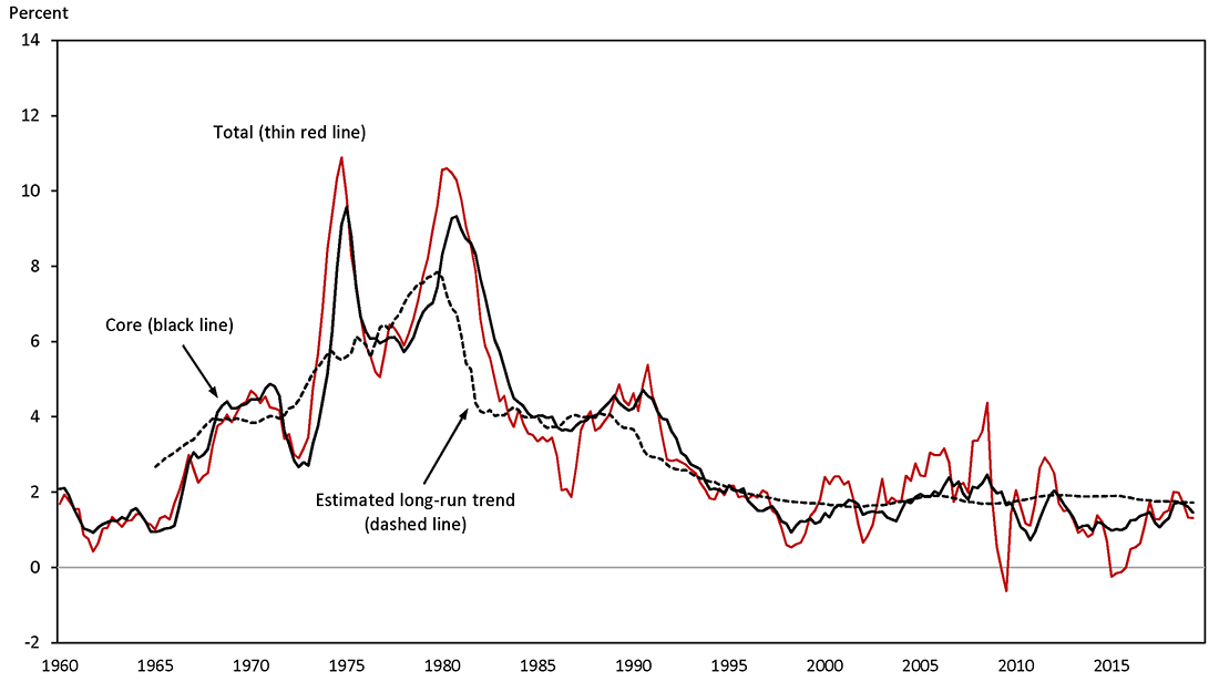
Note: Actual inflation computed as four‐quarter log difference of market‐based PCE price indexes. Estimated trend is from TVP‐VAR model with labor costs.
What might have caused inflation's long-run trend to become largely invariant to economic conditions after the mid-1990s? A potential explanation suggests itself if we compare the estimated trend with measures of long-run expected inflation from surveys, which is done in Figure 2. Both the contour and recent relative stability of trend inflation are roughly mirrored by the two survey measures shown in the figure (household expectations from the Michigan Survey, and inflation projections from the Survey of Professional Forecasters, or SPF).13 This observation has led some to conclude that better-anchored inflation expectations have ultimately been behind the change in this feature of the inflation process—though the evidence for this conclusion is circumstantial at best.14
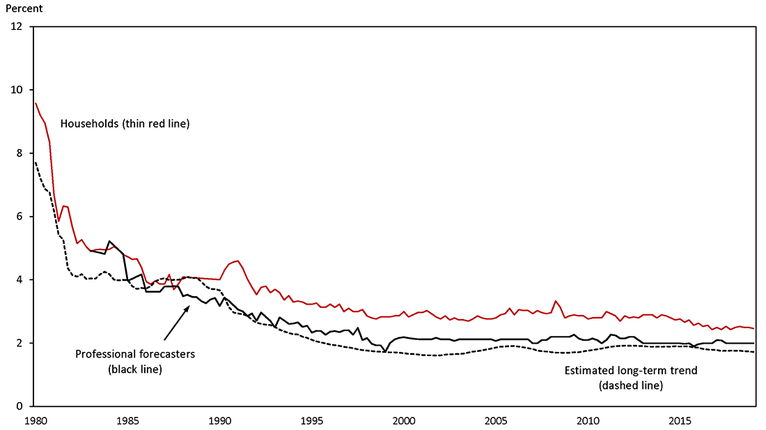
Note: Household expectations are median long‐term expectations from the University of Michigan Surveys of Consumers, with linear interpolation in selected periods prior to 1990:Q2. Expectations for professional forecasters are derived from the Federal Reserve Bank of Philadelphia's Survey of Professional Forecasters. Estimated trend is from TVP‐VAR model with labor costs.
As was mentioned earlier, the inclusion of a measure of labor costs in the VAR model necessitates using market-based PCE prices (see note 11). Although market-based prices account for nearly 90 percent of the full core PCE price index, if the nonmarket component tends to rise at a different rate, on average, than the remainder of the index, then we might be concerned that the estimate of trend inflation obtained from a model whose core inflation measure excludes nonmarket prices will not provide a correct measure of underlying inflation for the overall core (or, by extension, for the total PCE price index).
One way to evaluate this possibility is to compare the trends obtained from two alternative TVP‑VAR models, one of which uses total core PCE inflation, and one of which uses the market-based core measure (the VAR specifications are otherwise identical, and both omit the labor cost term).15 Lines 4 and 5 of Table 1 report the resulting trend inflation estimates; comparing the two sets of estimates indicates that the long-run trend in overall core inflation has tended to run about 0.1 percentage point above the market-based trend, which suggests in turn that the estimate of underlying inflation obtained from the wage-price VAR and shown in line 3 should be increased by a similar amount if we desire an estimate of underlying inflation for the overall core.16
Using survey expectations to estimate underlying inflation
The fact that the contour of these survey measures of long-run expected inflation appear to closely follow inflation's estimated long-run trend (perhaps up to a fixed wedge) suggests that we might use them directly to inform our estimate of underlying inflation.17 One way to do this is to fit an equation of the form:
$$ (4)\ \ \ \ \ \ \pi_t = (1-\phi)(\hat{\pi}^e_t + \lambda) + \phi \pi_{t-1} + \beta \tilde{U}_t + \gamma X_t + \varepsilon_t , $$
where $$\pi_t$$ is core PCE inflation, $$\hat{\pi}^e_t$$ is a survey measure of long-run expectations (plus a fixed wedge $$\lambda$$), $$\tilde{U_t}$$ and $$X_t$$ are, respectively, measures of slack and supply shocks, and $$\varepsilon_t$$ is a residual. This specification is similar to the expectations-augmented Phillips curve described by Yellen (2015), modified such that—absent slack and supply shocks, and with a fixed value of inflation expectations—inflation will converge to a long-run level that can differ from the inflation expectations measure by a constant amount.18 The specification can also be motivated from a model like equation (3), where we augment that equation to explicitly include measures of slack and supply shocks, assume a fixed autoregressive parameter $$\phi$$, and associate the time-varying mean of inflation with $$\hat{\pi}^e_t + \lambda$$. (In either case, this latter sum represents the model's estimate of underlying inflation.)
Estimating this model with the Michigan and SPF expectation measures yields the underlying inflation values shown in lines 6 and 7 of Table 1.19 The underlying inflation estimate from the Michigan-based model inherits the roughly ½ percentage point decline seen in this expectations measure over this period (and evident from Figure 2); the SPF-based estimate is more stable, but the presence of a small negative estimated wedge implies that its 2019:Q2 point value is 0.1 percentage point lower than the actual SPF expectation of 2 percent.
The plots in Figure 2 suggest that the assumption of a constant wedge between the Michigan expectations measure and trend inflation might not be a good one (and even the SPF measure manifests short-run movements that are not closely mirrored by the estimated inflation trend). More broadly, we might want to allow for the possibility that these survey measures are not perfectly correlated with trend inflation, perhaps because they actually are biased, or perhaps because they only provide imperfect proxies for the expectations that actually matter for price determination.
A model developed by Chan, et al. (2018) allows us to use measures of long-run expected inflation to inform estimates of trend inflation in a reasonably flexible way. Their approach starts with the autoregressive trend-deviation model of equation (2), and augments it with a second equation that assumes that an observed measure of long-run expected inflation $$\hat{\pi}^e_t$$ is a linear function of trend inflation,
$$\ \ \ \ \ \ \ \ \ \ \hat{\pi}^e_t = d_{0t} + d_{1t} \pi^{\ast}_t + \epsilon_t + \psi \epsilon_{t-1} , $$
with an intercept and slope that are allowed to vary over time (the equation also assumes an MA(1) process for the error term).
Trend inflation estimates from this model are shown in Table 1 for the Michigan expectations measure (line 8) and for the SPF (line 9). The decline in the Michigan-based trend is much smaller than that seen for the actual Michigan series; for the SPF measure, which has been close to flat over the past two decades, the trend inflation estimates are similar to those obtained from the time-varying AR model (line 2).
The table also presents results using a measure of 6-to-10-year-ahead breakeven inflation derived from TIPS yields, which some observers have argued provides a better read of private-sector long-run inflation expectations but which also might be affected by changes in inflation risk or Treasury liquidity premiums that are unrelated to changes in expected inflation.20 Since 2007:Q4, the actual decline in this series has been close to a percentage point; by contrast, the decline in the estimate of trend inflation obtained from the TIPS-based model is much smaller, on the order of ¼ percentage point (line 10).
Joint estimation of underlying inflation and economic slack
Up to this point, we have assumed that we know the "natural rate" of unemployment (defined here as the level of unemployment that corresponds to an absence of economic slack). In a single-equation setup such as a Phillips curve, we cannot separately identify underlying inflation and the natural rate: Any assumed value for the natural rate can be made consistent with a given realization of actual inflation by suitably adjusting the level of underlying inflation, and vice-versa.
Such joint estimation is possible, however, in a model that uses additional dynamic relationships to inform the estimate of the natural rate. Line 11 of Table 1 reports underlying inflation estimates obtained from such a model, which treats both the natural rate and underlying inflation as unobserved, and which then tries to infer their behavior based on their assumed relationship with various observed variables (specifications like these are often referred to as "state‑space models"). The underlying inflation estimates shown in line 11 come from a system with a relatively large number of dynamic relationships and observable variables; in 2019:Q2, this model's estimate lies within the range of values obtained from the other models.21
A broader conceptual issue
A conceptual issue that arises in trying to relate these various empirical estimates to our definition of underlying inflation concerns what it means for a supply shock—or economic slack—to be "absent." For example, since 1998 the change in the relative price of imports, which is used by the VAR and Phillips curve models to capture one type of supply shock, has been negative on average.22 We might therefore view a downward trend in relative import prices as a typical state of affairs, and hence one that is likely to prevail going forward. If so, then we would want to view a decline in relative import prices that is in line with this trend as corresponding to a situation in which this particular supply shock is "absent" for the purposes of our underlying inflation definition.23
Our definition of underlying inflation also requires economic slack to be absent.24 If we view that situation as one in which the state of resource utilization is putting neither upward nor downward pressure on inflation, then the correct benchmark to use for our definition of underlying inflation is one where contribution of slack to actual inflation is zero—even if such a state has not prevailed "on average" over history.25
With these considerations in mind, how well do the various estimates presented in Table 1 correspond to estimates of underlying inflation under our definition?
- To the extent that nonzero supply shocks—or a nonzero margin of economic slack—have persistently influenced actual inflation over history, then their effects will be captured by the trends from the univariate models. This situation is probably desirable in the case of supply shocks—in particular, the relative price trend that has prevailed in recent years for import prices likely provides a reasonable guess as to how these prices will evolve going forward. But it is probably a less-appealing situation in the case of slack: The CBO measure of the unemployment gap averages 0.7 percentage point from 1998:Q1 to 2019:Q2, suggesting that actual inflation rates over this period—and hence the trend estimates—also reflect a nonzero contribution from slack.26
- Similarly, the effects of these influences will likely be captured to some degree by the trend estimates from the Chan, et al. (2018) models that combine measures of long-run expected inflation with an autoregressive inflation gap equation, since the gap equation's trend estimates will also reflect the historical behavior of actual inflation.
- The underlying inflation estimate reported for the Phillips curve models specifically corresponds to the level of inflation that would eventually result if the unemployment gap and the rate of change of relative import prices were zero, and if the inflation expectations measure in the model were held fixed at its current level. Hence, if we define the influence of relative import prices to be "absent" when they are declining at some specified rate, we would need to adjust the model's estimate of underlying inflation accordingly so as to bring it conceptually into line with our definition.27
- In the case of the various TVP‑VAR models, the correspondence between the models' trend inflation estimate and the underlying inflation concept will be close, so long as we are willing to define a supply shock as being "absent" whenever its empirical analogue is equal to the VAR model's estimated long-run mean for that variable.28
- The underlying inflation estimate from the state-space model, like the Phillips curve estimates, is also defined as the inflation rate that is consistent with no unemployment gap and a zero rate of change of relative import prices.29 Moreover, to the extent that the estimate of slack from this model is mainly informed by the observed behavior of variables other than inflation, periods with a zero estimated unemployment gap need not exactly correspond to a state of the economy in which resource utilization is truly making no contribution to inflation (with any slippage likely showing up in the model's estimate of underlying inflation).
Finally, a related issue (which was alluded to in footnote 4) is that estimates of underlying core inflation such as those considered here will provide poor estimates of underlying total inflation if we expect that relative food and energy prices will make a nonzero contribution to total inflation going forward. As an empirical matter, from 1998:Q1 to 2019:Q2 food and energy prices have caused total PCE price inflation to run 0.1 percentage point per year above core PCE inflation on average. However, this average contribution of food and energy prices is statistically indistinguishable from zero.
Some implications for policy suggested by these estimates
The estimates of underlying inflation shown in Table 1 have two noteworthy features, both of which are potentially relevant for monetary policy.
Most obviously, the estimates for the most-recent period are, without exception, below the Federal Reserve's longer-run inflation goal of 2 percent. Taken at face value, these estimates suggest that it will not be possible to achieve that 2 percent goal unless resource utilization is kept at a level high enough to make a sustained positive contribution to inflation (or unless the behavior of other influences on inflation, such as import prices, turns out to be markedly different from past experience). Of course, some estimates are closer to 2 percent than others (especially once statistical uncertainty is taken into account), and it would be useful to determine which model's estimate is most likely to be correct. Unfortunately, one natural criterion—namely, which model does the best job of forecasting actual inflation—does not seem to be especially informative.30
Second, to the extent that the remarkable stability of these estimates over the past two decades reflects a durable feature of the inflation process, it offers a significant boon to policymakers—as Yellen (2015) notes, such a situation "greatly enhances a central bank's ability to pursue both of its objectives—namely, price stability and full employment." That said, our understanding of the source of this stability is exceedingly tenuous (as is our understanding of what has caused other changes in inflation dynamics, such as the apparent attenuation over time of the relationship between inflation and slack). It is therefore difficult to claim much certainty regarding how any features of the inflation process will evolve going forward—and, hence, whether they can be relied on by policymakers.
References
Beveridge, Stephen, and Charles R. Nelson (1981). "A New Approach to Decomposition of Economic Time Series into Permanent and Transitory Components with Particular Attention to Measurement of the 'Business Cycle'." Journal of Monetary Economics, 7, 151–174.
Blinder, Alan S., and Jeremy B. Rudd (2013). "The Supply-Shock Explanation of the Great Stagflation Revisited." In The Great Inflation: The Rebirth of Modern Central Banking, edited by Michael D. Bordo and Athanasios Orphanides, pp. 119–75. Chicago: University of Chicago Press.
Chan, Joshua C. C., Todd E. Clark, and Gary Koop (2018). "A New Model of Inflation, Trend Inflation, and Long-Run Inflation Expectations." Journal of Money, Credit and Banking, 50, 5–53.
Clark, Todd E., and Taeyoung Doh (2014). "Evaluating Alternative Models of Trend Inflation." International Journal of Forecasting, 30, 426–448.
Clark, Todd E., and Stephen J. Terry (2010). "Time Variation in the Inflation Passthrough of Energy Prices." Journal of Money, Credit and Banking, 42, 1419–33.
Cogley, Timothy, Giorgio E. Primiceri, and Thomas J. Sargent (2010). "Inflation-Gap Persistence in the US." American Economic Journal: Macroeconomics, 2, 43–69.
Fieller, E. C. (1954). "Some Problems in Interval Estimation." Journal of the Royal Statistical Society Series B (Methodological), 16, 175–185.
Peneva, Ekaterina V., and Jeremy B. Rudd (2017). "The Passthrough of Labor Costs to Price Inflation." Journal of Money, Credit and Banking, 49, 1777–1802.
Sargent, Thomas J. (1987). Macroeconomic Theory. Boston: Academic Press.
Staiger, Douglas, James H. Stock, and Mark W. Watson (1997). "How Precise Are Estimates of the Natural Rate of Unemployment?" In Reducing Inflation: Motivation and Strategy, edited by Christina D. Romer and David H. Romer, pp. 195–242. Chicago: University of Chicago Press.
Stock, James H., and Mark W. Watson (2007). "Why Has U.S. Inflation Become Harder to Forecast?" Journal of Money, Credit and Banking, 39(S1), 3–33.
Yellen, Janet L. (2015). "Inflation Dynamics and Monetary Policy." (Remarks given as the September 24, 2015 Phillip Gamble Memorial Lecture, University of Massachusetts, Amherst.)
1. [email protected]; Board of Governors of the Federal Reserve System, Research and Statistics Division, Washington, DC 20551. I would like to thank Travis Berge, Rochelle Edge, Andrew Figura, David Lebow, Matteo Luciani, Christopher Nekarda, and Ekaterina Peneva for various useful conversations and helpful comments on an earlier draft. (The usual caveat applies.) This note reflects my own views and does not indicate concurrence by other members of the research staff or the Board of Governors. Return to text
2. The term "underlying inflation" is sometimes used to describe the measurement goal of certain price indexes, such as median or trimmed-mean measures or exclusion indexes, that attempt to reduce the influence of idiosyncratic relative price movements. This alternative definition of underlying inflation is distinct to the one considered here. Return to text
3. As I discuss below, I actually consider two separate variants of core PCE inflation (namely, the overall core measure and a core measure that excludes nonmarket PCE prices). Return to text
4. Conceptually, there will be no difference between underlying inflation defined with respect to core PCE prices and underlying inflation defined in terms of total PCE prices if we view changes in relative food and energy prices as purely idiosyncratic in nature or if we define them to be supply shocks. (As a matter of accounting, the rate of total PCE price inflation equals the rate of core PCE inflation plus the weighted sum of changes in the relative prices of food and energy, where "relative" here means "relative to core" and where the weights are the relevant expenditure shares.) Return to text
5. If the variance of $$\eta$$ were constant (that is, if we assumed a white-noise process for $$\eta$$ rather than allowing it to exhibit stochastic volatility), then trend inflation would follow a random walk. Return to text
6. An equation like (3) can be derived by setting $$\pi^{\ast}_{t-1} = \pi^{\ast}_t$$![]() on the right-hand side of equation (2), and then rearranging terms. A specification similar to (3), with the parameters $$\mu$$ and $$\phi$$ assumed to follow random walks and with stochastic volatility for the error term $$e$$, is examined in the on-line appendix to Cogley, et al. (2010). Return to text
on the right-hand side of equation (2), and then rearranging terms. A specification similar to (3), with the parameters $$\mu$$ and $$\phi$$ assumed to follow random walks and with stochastic volatility for the error term $$e$$, is examined in the on-line appendix to Cogley, et al. (2010). Return to text
7. When the specification contains additional lags, so that $$\pi_t = \mu_t + \phi_{1,t} \pi_{t-1} + \phi_{2,t} \pi_{t-2} + \dots + \phi_{p,t} \pi_{t-p} + \varepsilon_t$$, the long-run mean will equal $$\mu_t/(1 - \phi_{1,t} - \phi_{2,t} - \dots - \phi_{p,t})$$. Return to text
8. The models are estimated over the period 1960:Q1–2019:Q2 using a core PCE price inflation series that removes Blinder and Rudd's (2013) estimates of the effects of the Nixon-era price controls and that also adjusts for the effect of the swing in measured insurance prices that resulted from the 9/11 terrorist attacks. The time-varying AR model includes two lags of inflation. Return to text
9. The two models' trend estimates are less similar earlier in the sample (not shown), likely reflecting changes in inflation persistence over time that the AR model is better able to control for. In particular, until the early 1980s the Stock–Watson trend estimate tracks high-frequency movements in actual inflation relatively closely, while the trend from the time-varying AR model is smoother. Return to text
10. This estimate corresponds to a stochastic trend for inflation in the sense of Beveridge and Nelson (1981). Return to text
11. The data used are updated versions of the series described in Peneva and Rudd (2017) and used in their full-sample VAR model (following those authors, inflation is measured using market-based core PCE prices to deal with the issue that prices for several nonmarket components of PCE are derived from wage or compensation measures). The estimation algorithm, which allows for stochastic volatility in the VAR innovations, is taken from Clark and Terry (2010); the sample period runs from 1965:Q1 to 2019:Q2. Return to text
12. See Peneva and Rudd (2017) for a discussion of the former channel, and Blinder and Rudd (2013) for a discussion of the latter. We might also view shocks to labor costs as representing a form of supply shock (for example, in a textbook AS/AD model exogenous changes in the money wage shift the AS curve—see Sargent, 1987, section II.3). Return to text
13. The SPF measure splices the median expectation for PCE inflation (which is available starting in 2007:Q1) to the median expectation for CPI inflation using the procedure described in Peneva and Rudd (2017). The Michigan measure is linearly interpolated in selected periods prior to 1990:Q2. Return to text
14. In particular, if some other aspect of the inflation process is responsible for the emergence of a stable long-run inflation trend, then the causality could run in the other direction, with the stable trend leading agents to anticipate a roughly constant long-run average rate of inflation. Return to text
15. I replace the labor cost series with share-weighted changes in relative energy prices (energy price increases were an important source of supply shocks in the 1970s and early 1980s). As in the previous exercise, the models also include a measure of the unemployment gap and a relative import price term; likewise, overall core PCE price inflation is again adjusted for the effects of the Nixon-era price controls and 9/11‑related insurance price swings. Return to text
16. Although the VARs whose results are shown in lines 3 and 5 of Table 1 both use market-based PCE prices, they need not yield the same trend estimates for inflation because their specifications differ in other regards. Return to text
17. A persistent level differential between the Michigan Survey expectation and the estimated long-run trend for PCE inflation need not imply that households' forecasts are biased, as the Michigan Survey does not ask respondents to report expectations for a specific price index but rather asks "[b]y about what percent per year do you expect prices to go (up/down) on the average, during the next 5 to 10 years?" While the SPF expectation does specifically correspond to the PCE price index (the survey question asks about "…annual average PCE inflation over the next 10 years"), this estimate could also differ from underlying (core) PCE inflation if SPF respondents expect changes in relative food and energy prices to make a nonzero average contribution to total PCE inflation over the long run. Return to text
18. The presence of a long-run expectations term in equation (4) would seem to be at odds with a traditional (Phelps–Friedman) Phillips curve in which the relevant expectation is $$E_{t-1} \pi_t$$ (that is, last period's expectation of the time‑$$t$$ inflation rate—a shorter‑run expectations concept). It is possible to show, however, that if agents use a simple autoregressive rule to generate their forecasts of inflation, then an equation like (4) will obtain from a Phelps–Friedman specification. In addition, the long-run expectation (which reflects the long-run mean for inflation implied by the forecasting rule) will be time-varying if agents revise their forecasting rule over time. Return to text
19. The model is estimated over the 1988:Q1 to 2019:Q2 period, and includes a relative import price term to control for supply shocks and an unemployment gap to capture slack (the variable definitions are the same as those used in the TVP-VAR models). In addition, the estimated version of the model lags the survey expectation measure by one quarter to ensure that it does not include the effect of any time-$$t$$ price changes. Finally, the confidence intervals shown in Table 1 for the resulting underlying inflation estimates are estimated using the application of Fieller's (1954) methodology proposed by Staiger, et al. (1997). Return to text
20. These TIPS-derived breakeven inflation data are available starting in 1999. Return to text
21. The state-space model considered here is a modified version of the supply block of the Federal Reserve Board's FRB/US model. Note that in 2019:Q2 the state-space model's estimate of the natural rate is 4.9 percent; the natural rate used by the other models—which is the CBO's estimate as of August 2019—equals 4.6 percent in 2019:Q2. Return to text
22. Specifically, from 1998:Q1 to 2019:Q2 the change in the measure of import prices used in these models has been 1.4 percentage points per year less rapid than the change in overall core PCE prices, and 1.3 percentage points less rapid than the change in market-based core prices. (The differential partly reflects the fact that imports are more heavily weighted toward goods, while PCE is more heavily weighted toward services.) Return to text
23. In principle, the same consideration applies to any supply shock that we might view as relevant for core inflation, such as changes in relative energy prices. However, results from various empirical models suggest that in recent years, changes in relative import prices have played a dominant role in this regard. Return to text
24. We take as given that we can correctly measure the margin of slack that is relevant for price determination. Return to text
25. A nonzero average level of slack could obtain, for example, if historically the economy has only tended to reach a full-utilization state at the end of the expansion phase of a business cycle. Return to text
26. Using the parameter estimates from the Phillips curve models as a rough guide, a persistent unemployment gap of this size would be expected to subtract a little less than 0.1 percentage point from annualized core PCE inflation. Return to text
27. For example, the parameter estimates from these models imply that we would want to reduce their underlying inflation estimates by a little less than 0.2 percentage point if we viewed a decline in relative import prices of 1.4 percent per year as typical. (Note that doing so would bring the SPF-based Phillips curve's estimates closer into line with the estimates from the SPF-augmented AR inflation gap model, whose trend likely already reflects the effect of declining relative import prices over history.) Return to text
28. In addition, the VAR's estimated long-run mean for the unemployment gap would need to be zero. (In the VAR models considered here, these long-run means are close enough to zero in recent years that they do not appear to be making much contribution to the estimated long-run mean for inflation.) Return to text
29. The state-space model also includes a relative energy price term in its inflation equation, so its underlying inflation definition assumes a zero rate of change of relative energy prices as well. Return to text
30. See Clark and Doh (2014). Return to text
Rudd, Jeremy B. (2020). "Underlying Inflation: Its Measurement and Significance," FEDS Notes. Washington: Board of Governors of the Federal Reserve System, September 18, 2020, https://doi.org/10.17016/2380-7172.2624.
Disclaimer: FEDS Notes are articles in which Board staff offer their own views and present analysis on a range of topics in economics and finance. These articles are shorter and less technically oriented than FEDS Working Papers and IFDP papers.