Policy Rules and How Policymakers Use Them
Alternative policy rules
While the Taylor rule is the best-known formula that prescribes how policymakers should set and adjust the short-term policy rate in response to the values of a few key economic variables, many alternatives have been proposed and analyzed.
The table below reports five policy rules that are illustrative of the many rules that have received attention in the academic research literature.1
| Taylor rule: | $$ R_t^T = r_t^{LR} + \pi_t + 0.5(\pi_t - \pi^*) + 0.5(y_t - y_t^P) $$ |
| Balanced-approach rule: | $$ R_t^{BA} = r_t^{LR} + \pi_t + 0.5(\pi_t - \pi^*) + (y_t - y_t^P) $$ |
|---|---|
| ELB-adjusted rule: | $$ R_t^{Eadj} = maximum \{ R_t^{BA} - Z_t, ELB \} $$ |
| Inertial rule: | $$ R_t^I = 0.85R_{t-1} + 0.15[r_t^{LR} + \pi_t + 0.5(\pi_t - \pi^*) + (y_t - y_t^P)] $$ |
| First-difference rule: | $$ R_t^{FD} = R_{t-1} + 0.1(\pi_t - \pi^*) + 0.1(y_t - y_{t-4}) $$ |
Note: ELB is a constant corresponding to the effective lower bound for the federal funds rate. $$ R_t^T$$, $$ R_t^{BA}$$, $$ R_t^{Eadj}$$, $$ R_t^I$$, and $$ R_t^{FD}$$ represent the values of the nominal federal funds rate prescribed by the Taylor, balanced-approach, ELB-adjusted, inertial, and first-difference rules, respectively. $$ R_t$$ denotes the actual federal funds rate for quarter $$ t$$; $$ r_t^{LR}$$ is the level of the neutral inflation-adjusted federal funds rate in the longer run that, on average, is expected to be consistent with sustaining inflation at 2 percent and output at its full resource utilization level; $$ \pi_t$$ is the four-quarter price inflation for quarter $$ t$$; $$ \pi^*$$ is the inflation objective, set at 2 percent; $$ y_t$$ is the log of real gross domestic product (GDP) in quarter $$ t$$; and $$ y_t^P$$ is the log of real potential GDP in quarter $$ t$$. Under the ELB-adjusted rule, the term $$ Z_t$$ is the cumulative sum of past deviations of the federal funds rate from the prescriptions of the balanced-approach rule when that rule prescribes setting the federal funds rate below zero.
All of the rules in the table prescribe a level for the policy rate that is related to the deviation of inflation from the central bank's objective--2 percent in the United States. The first four rules also respond to the percentage difference between the current value of real gross domestic product (GDP) and potential GDP. These rules differ in terms of how strongly the prescribed policy rate reacts to the inflation and resource utilization gaps. The third rule recognizes that there is an effective lower bound (ELB) on the policy rate; in practice, central banks have judged that the ELB is close to zero.2 This rule tracks the balanced-approach rule during normal times, but after a period during which the balanced-approach rule prescribes setting the policy rate below the ELB, the ELB-adjusted rule keeps the policy rate low for a long enough time to make up for the past shortfall in accommodation. The fourth and fifth rules differ from the other rules in that they relate the current policy prescription to the level of the policy rate in the previous period. The final rule responds to the change in real GDP rather than the percentage deviation of real GDP from potential GDP.
A detailed discussion of the Taylor rule formula is provided in Principles for the Conduct of Monetary Policy. The balanced-approach rule is similar to the Taylor rule except that the coefficient on the resource utilization gap is twice as large as in the Taylor rule.3 Thus, this rule puts more weight on stabilizing that gap than does the Taylor rule--a distinction that becomes especially important in situations in which there is a conflict between inflation stabilization and output-gap stabilization. An example is when inflation is above the 2 percent objective by the same amount that output is below its full resource utilization level. In this situation, the balanced-approach rule prescribes a lower federal funds rate than the Taylor rule because the balanced-approach rule places a higher weight on providing the monetary stimulus necessary to raise the level of output up to its full resource utilization level.
When inflation is running well below 2 percent and there is substantial slack in resource utilization, some policy rules prescribe setting the federal funds rate materially below zero; doing so is not feasible. The ELB-adjusted rule recognizes this constraint and thus prescribes setting the policy rate at the ELB whenever the balanced-approach rule prescribes a rate below the ELB. The term $$ Z_t$$ measures the cumulative shortfall in monetary stimulus that occurs because short-term interest rates cannot be reduced below the ELB. Compared with the balanced-approach rule, the ELB-adjusted rule would leave the federal funds rate lower for a longer period of time following an episode when the balanced-approach rule would prescribe policy rates below the ELB.
The inertial rule prescribes a response of the federal funds rate to economic developments that is spread out over time. For example, the response to a persistent upside surprise to inflation would gradually build over time, and the federal funds rate would ultimately rise to the same level as under the balanced-approach rule.4 This kind of gradual adjustment is a feature often incorporated into policy rules; it damps volatility in short-term interest rates. Some authors have argued that such gradualism describes how the Federal Reserve has implemented adjustments to the federal funds rate historically or how inertial behavior can be advantageous--for example, because it allows stabilizing the economy with less short-term interest rate volatility.5
The first-difference rule, like the inertial rule, relates the current value of the federal funds rate to its previous value. One feature of this rule is that it does not require information about the value of the neutral real policy rate in the longer run or about the level of output at full resource utilization. Instead, under the first-difference rule, the prescribed change in the federal funds rate depends only on inflation and output growth.6 Advocates of this rule emphasize that both the neutral real federal funds rate in the longer run and the level of GDP associated with full resource utilization are unobserved variables that likely vary over time and are estimated with considerable uncertainty. In light of these difficulties, they prefer rules like the first-difference rule in which the prescriptions for the change in the federal funds rate do not depend on estimates of unobserved variables.7 Moreover, these advocates have emphasized that the first-difference rule, similar to the other rules, stabilizes economic fluctuations so that inflation converges to its objective over time and output converges to a level consistent with full resource utilization. This feature reflects that the first-difference rule satisfies the key principles of good monetary policy discussed in Principles for the Conduct of Monetary Policy; in particular, it calls for the policy rate to rise over time more than one-for-one in response to a sustained increase in inflation.
Fed policymakers consult, but do not mechanically follow, policy rules
Policy rules provide useful benchmarks for setting and assessing the stance of monetary policy. Well-specified rules are appealing because they incorporate the key principles of good monetary policy discussed in Principles for the Conduct of Monetary Policy, but they nevertheless have shortcomings.
In deciding how to set monetary policy, the Federal Open Market Committee (FOMC) regularly consults the policy prescriptions from several monetary policy rules along with other information that is relevant to the economy and the economic outlook.8 Because of the small number of variables in these rules, the rules are easy to interpret and they provide a starting point for thinking about the implications of incoming information for the level of the federal funds rate. Despite their apparent simplicity, these rules raise a number of issues if they were to be used to implement monetary policy. If policymakers wanted to follow a policy rule strictly, they would have to determine which measure of inflation should be used (for example, they could choose the rate at which the consumer price index is rising, the growth rate of the price index for personal consumption expenditures, inflation measures net of food and energy price inflation, or even measures of wage inflation) and which measure of economic activity should be used (for example, output relative to its level at full resource utilization, the deviation of the unemployment rate from its longer-run average level, or the growth rates of these variables). The value of the neutral real federal funds rate in the longer run would need to be determined, and policymakers would need to decide whether that rate is varying over time and, if so, in what manner .
The U.S. economy is highly complex, however, and monetary policy rules, by their nature, do not capture that complexity. This complexity reflects in part the ever-changing nature of the U.S. economy in response to a variety of factors that lead to resource reallocations across sectors. (Such factors include demographic developments, new technologies, and other shifts that occur over time and are not related to monetary policy.) These changes in the economy make it difficult to accurately measure variables that are important determinants of the rules--such as potential output, the natural rate of unemployment, and the neutral real federal funds rate in the longer run--as well as to disentangle the effects of permanent and transitory changes on the economy. Consequently, the FOMC examines a great deal of information to assess how realized and expected economic conditions are evolving relative to the objectives of maximum employment and 2 percent inflation. As discussed in Challenges Associated with Using Rules to Make Monetary Policy, there are important limitations that argue against mechanically following any rule.
Because the U.S. economy is complex and the understanding of it is incomplete, Fed policymakers have a diversity of views about some of the details of how monetary policy works and how the federal funds rate should be adjusted to most effectively promote maximum employment and price stability. These differing views are reflected in the economics profession more generally and in alternative formulations of policy rules.
As shown in figure 1, historical prescriptions from policy rules differ from one another and also differ from the actual level of the federal funds rate (the black solid line).9 Although the prescriptions of the five rules tend to move up and down together over time, there can be significant differences in the levels of the federal funds rate that these rules prescribe. The prescriptions of the inertial rule and the first-difference rule typically call for more gradual adjustments of the federal funds rate than the prescriptions from the Taylor rule and the balanced-approach rule.
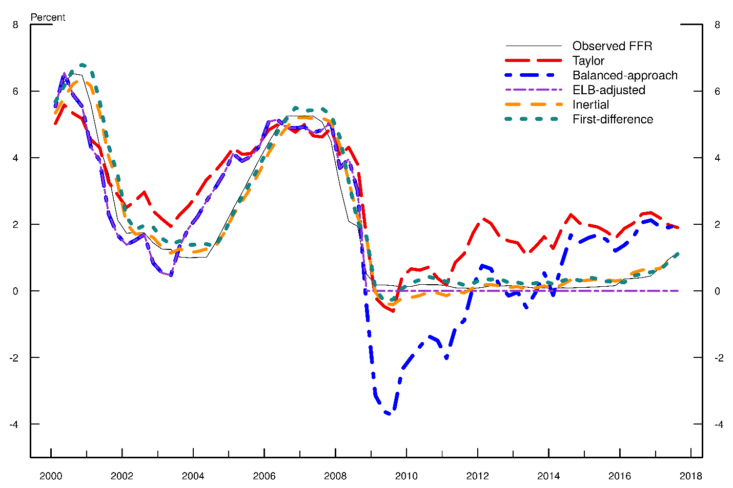
Note: To calculate rule prescriptions, inflation is measured as the four-quarter log difference of the quarterly average of the price index for personal consumption expenditures excluding food and energy. The output gap is measured as the log difference between real gross domestic product (GDP) and potential real GDP. The level of the neutral inflation-adjusted federal funds rate in the longer run, $$ r_t^{LR}$$, is measured as the difference between the linearly interpolated quarterly average values of the long-term forecast for the three-month Treasury bill rate and the long-term forecast for inflation of the implicit GDP price deflator from Blue Chip Economic Indicators. ELB stands for effective lower bound, and FFR stands for federal funds rate. For descriptions of the simple rules, see the text.
Source: The following data series were retrieved from FRED, Federal Reserve Bank of St. Louis: Federal Reserve Board, effective federal funds rate [FEDFUNDS]; Bureau of Economic Analysis, personal consumption expenditures excluding food and energy (chain-type price index) [PCEPILFE], real gross domestic product [GDPC1]; and Congressional Budget Office, real potential gross domestic product [GDPPOT]. In addition, data were drawn from Wolters Kluwer, Blue Chip Economic Indicators.
Figure 1 also shows that all of the rules called for a significant reduction in the federal funds rate in 2008, when the U.S. economy deteriorated substantially during the Global Financial Crisis. In addition, all of the rules, except for the ELB-adjusted rule, called for values of the policy rate that were below the ELB in 2009.10 The rates prescribed by the balanced-approach rule were substantially below zero, reflecting the appreciable shortfalls in real GDP from its full resource utilization level in 2009 and 2010 and this rule's large coefficient on those deviations. As the economy recovered and real GDP moved back toward its potential level, the prescriptions given by the Taylor and the balanced-approach rules rose and moved well above zero by 2015. However, the prescriptions of the inertial and first-difference rules increased more gradually in response to the improvement in economic conditions, and they remained persistently low for several years after 2009.
The large discrepancies between the actual federal funds rate and the prescriptions given by the Taylor rule and the balanced-approach rule suggest that economic outcomes likely would have been significantly different had monetary policy followed one of these rules. To address questions such as these, economists use models of the U.S. economy designed to evaluate the implications of alternative monetary policies. However, these models are invariably simplifications of reality, and there is no agreed-upon "best" model representation of the U.S. economy. Without wide agreement on the metric for evaluating alternative policy rules, there remains considerable debate among economists regarding the merits and shortcomings of the various rules.
1. The Taylor rule was suggested in John B. Taylor (1993), "Discretion versus Policy Rules in Practice," Carnegie-Rochester Conference Series on Public Policy, vol. 39 (December), pp. 195-214. The balanced-approach rule was analyzed in John B. Taylor (1999), "A Historical Analysis of Monetary Policy Rules," in John B. Taylor, ed., Monetary Policy Rules (Chicago: University of Chicago Press), pp. 319-41. The ELB-adjusted rule was studied in David Reifschneider and John C. Williams (2000), "Three Lessons for Monetary Policy in a Low-Inflation Era," Journal of Money, Credit, and Banking, vol. 32 (November), pp. 936-66. Finally, the first-difference rule is based on a rule suggested by Athanasios Orphanides (2003), "Historical Monetary Policy Analysis and the Taylor Rule," Journal of Monetary Economics, vol. 50 (July), pp. 983-1022. A comprehensive review of policy rules is in John B. Taylor and John C. Williams (2011), "Simple and Robust Rules for Monetary Policy," in Benjamin M. Friedman and Michael Woodford, eds., Handbook of Monetary Economics, vol. 3B (Amsterdam: North-Holland), pp. 829-59. The same volume of the Handbook of Monetary Economics also discusses approaches other than policy rules for deriving policy rate prescriptions. Return to text
2. Some foreign central banks have demonstrated that it is possible to make short-term interest rates modestly negative. Return to text
3. For an articulation of the view that this rule is more consistent with following a balanced approach to promoting the Federal Open Market Committee's dual mandate than is the Taylor rule, see Janet L. Yellen (2012), "The Economic Outlook and Monetary Policy," speech delivered at the Money Marketeers of New York University, New York, April 11. Return to text
4. This example assumes that the prescriptions of the balanced-approach and inertial rules for the federal funds rate do not incorporate feedback effects on the macroeconomy that influence the behavior of real GDP, unemployment, inflation, and other variables. If the rule prescriptions did incorporate such feedback effects, then the macroeconomic outcomes could differ significantly over time between the two rules because these rules prescribe different interest rate paths in the near term. Return to text
5. Authors William English, William Nelson, and Brian Sack discuss several reasons why policymakers may prefer to adjust rates sluggishly in response to economic conditions. The authors emphasize that such a response may be optimal in the presence of uncertainty about the structure of the macroeconomy and the quality of contemporaneous data releases, as well as the fact that policymakers may be concerned that abrupt policy changes could have adverse effects on financial markets if those changes confused market participants. See William B. English, William R. Nelson, and Brian P. Sack (2003), "Interpreting the Significance of the Lagged Interest Rate in Estimated Monetary Policy Rules," B.E. Journal of Macroeconomics, vol. 3 (April), pp. 1-18. For a discussion of the motives for interest rate smoothing and its role in U.S. monetary policy, see Ben S. Bernanke (2004), "Gradualism," speech delivered at an economics luncheon cosponsored by the Federal Reserve Bank of San Francisco (Seattle Branch) and the University of Washington, Seattle, May 20. Return to text
6. For a discussion of the properties of the first-difference rule, see Athanasios Orphanides and John C. Williams (2002), "Robust Monetary Policy Rules with Unknown Natural Rates (PDF)," Brookings Papers on Economic Activity, no. 2, pp. 63-118. Return to text
7. Although the first-difference rule does not require estimates of the neutral real federal funds rate in the longer run or the level of potential output, this rule has drawbacks. For example, research suggests that rules of this type will typically create greater variability in employment and inflation than what would prevail under the Taylor and the balanced-approach rules, unless policymakers' estimates of the neutral real federal funds rate in the longer run and the level of potential output are seriously in error. Return to text
8. Federal Reserve staff regularly report the prescriptions from simple rules to the FOMC in the Report to the FOMC on Economic Conditions and Monetary Policy (also known as the Tealbook), which is prepared before each FOMC meeting. The prescriptions of the Taylor, balanced-approach, and first-difference rules as well as other rules were discussed, for instance, in the most recent publicly available report, which can be found on the Board's website at https://www.federalreserve.gov/monetarypolicy/files/FOMC20111213tealbookb20111208.pdf. Return to text
9. The figure does not take into account the fact that, had the FOMC followed one of the policy rules presented there, the outcomes for inflation and real GDP could have differed significantly from those observed in practice, in turn making the rule prescriptions different from those shown in the figure. However, Federal Reserve Board staff regularly use economic models of the U.S. economy (1) to study how economic outcomes could change if monetary policy were to follow some rule and (2) to compute rule prescriptions taking this endogenous feedback into consideration. These so-called dynamic simulations also show marked differences in prescribed paths for the federal funds rate and resulting paths for inflation, real GDP, and labor market variables. Return to text
10. To provide additional stimulus when the federal funds rate was near the ELB, the FOMC purchased longer-term securities in order to put downward pressure on longer-term interest rates. In addition, the FOMC in its communications provided guidance that it planned to keep its target for the federal funds rate unchanged. Return to text