FEDS Notes
November 09, 2020
Updating the Distributional Financial Accounts
Michael Batty, Eric Nielsen, Kamila Sommer, Alice Volz, Sarah Friedman, Ella Deeken, Jesse Bricker, and Sarah Reber
In addition to incorporating 2020q2 data from the Financial Accounts, the 2020q2 release of the Distributional Financial Accounts (DFAs) includes three substantial updates. The most consequential is the incorporation of the newly released 2019 Survey of Consumer Finances (SCF). Additionally, there are two technical updates to the temporal disaggregation method we use to interpolate and extrapolate distributional information for the quarters between and beyond the triennial SCF releases. This note first describes these changes, and then highlights how they have affected several aspects of the DFA data. We also discuss developments in wealth inequality in the quarters since the 2019 SCF. For a full description of the DFA data and methodology, see Batty et. al. (2020).
2019 Survey of Consumer Finances
The most important difference between the 2020q2 DFA release and the 2020q1 release is the incorporation of the 2019 SCF, which was publicly released on September 28, 2020.1 Previous DFA releases were based on SCF data that ended in 2016, and thus each quarter of DFA data after 2016q3 was extrapolated using our temporal disaggregation model in the 2020q1 release. The DFA data are now based upon all the SCF data from 1989 through 2019. The quarters between 2016q3 and 2019q3 are now interpolated between the 2016 and 2019 SCFs, while the quarters after 2019q3 are extrapolated using data from the Financial Accounts and other sources.
Incorporating the 2019 SCF has two distinct effects on the DFAs. First, it provides direct evidence on how the wealth distribution has evolved since the 2016 SCF. Second, it provides new data that inform the temporal disaggregation methodology we use to interpolate between SCF surveys. The resulting adjustments to the estimated relationships underlying this methodology, in turn, produce more subtle changes over the history of the DFAs.2
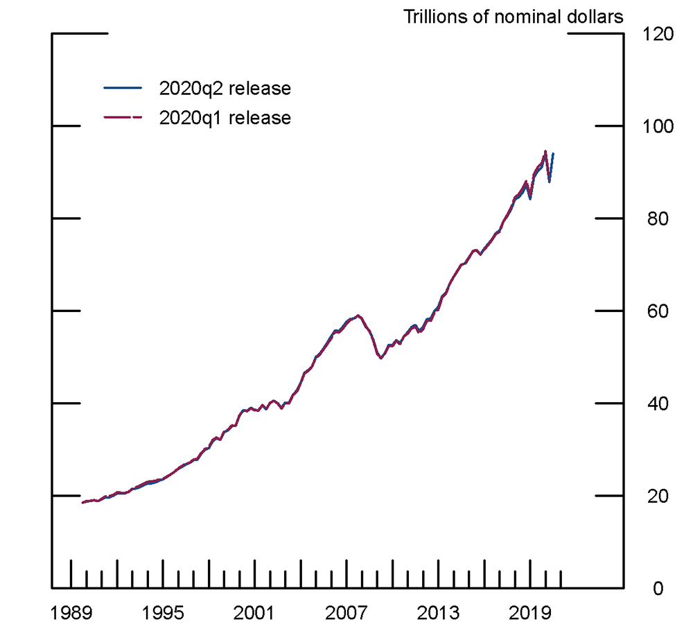
Before discussing the other updates, we note that the new data provide a fresh opportunity to assess the comparability of the SCF and the Financial Accounts, which use different methods and data to provide measures of aggregate household wealth. The new SCF data show that these two sources of information on household wealth continue to align well in the aggregate. Aggregate net worth in the 2019 SCF is about three percent larger than in the Financial Accounts in 2019q3. This is a closer match than on the 12 percent difference observed for the 2016 SCF, and near to the average 4 percent difference over the 11 SCF surveys since 1989. Importantly, the individual asset and liability totals remain generally quite close as well. In fact, Table 1 shows that for almost all balance-sheet items, the difference between the SCF and Financial Accounts fell between 2016 and 2019.
Table 1: The Ratio of the Reconciled SCF Household Balance Sheet to B.101.h
| Ratios in SCF Years | Recent Levels ($ billion) | |||||||||||||
|---|---|---|---|---|---|---|---|---|---|---|---|---|---|---|
| 1989 | 1992 | 1995 | 1998 | 2001 | 2004 | 2007 | 2010 | 2013 | 2016 | 2019 | Average | FA 2019Q3 | SCF 2019 | |
| Total Assets | 97 | 91 | 91 | 97 | 108 | 104 | 102 | 106 | 102 | 108 | 101 | 101 | 123097 | 124778 |
| Nonfinancial assets | 97 | 92 | 91 | 99 | 97 | 105 | 113 | 117 | 115 | 110 | 106 | 104 | 35329 | 37335 |
| Real estate (1) | 107 | 105 | 101 | 110 | 105 | 113 | 123 | 131 | 127 | 119 | 114 | 114 | 29612 | 33644 |
| Consumer durable goods (2) | 60 | 48 | 58 | 58 | 64 | 67 | 63 | 62 | 63 | 66 | 65 | 61 | 5717 | 3690 |
| Financial assets | 98 | 91 | 91 | 97 | 114 | 103 | 96 | 100 | 98 | 107 | 100 | 100 | 87767 | 87443 |
| Checkable deposits and currency | 65 | 45 | 50 | 85 | 136 | 194 | 809 | 240 | 130 | 145 | 194 | 190 | 796 | 1541 |
| Time deposits and short-term investments | 60 | 63 | 59 | 65 | 58 | 63 | 51 | 54 | 42 | 47 | 45 | 55 | 9779 | 4431 |
| Money market fund shares | 83 | 80 | 76 | 59 | 73 | 101 | 71 | 93 | 133 | 128 | 102 | 91 | 1968 | 2003 |
| U.S. government and municipal securities | 70 | 53 | 54 | 54 | 106 | 95 | 94 | 72 | 82 | 101 | 76 | 78 | 4497 | 3413 |
| Corporate and foreign bonds | 88 | 51 | 27 | 31 | 69 | 61 | 60 | 45 | 64 | 108 | 95 | 64 | 774 | 738 |
| Other loans and advances | 333 | 123 | 186 | 63 | 62 | 43 | 34 | 52 | 71 | 54 | 62 | 98 | 789 | 491 |
| Mortgages | 110 | 94 | 91 | 84 | 97 | 97 | 102 | 96 | 177 | 275 | 213 | 131 | 59 | 125 |
| Corporate equities and mutual fund shares | 144 | 120 | 121 | 132 | 187 | 142 | 112 | 128 | 111 | 129 | 112 | 131 | 26550 | 29743 |
| Life insurance reserves | 100 | 100 | 100 | 100 | 100 | 100 | 100 | 100 | 100 | 100 | 100 | 100 | 1719 | 1715 |
| Pension entitlements (3) | 101 | 100 | 100 | 100 | 100 | 100 | 100 | 100 | 100 | 100 | 100 | 100 | 27279 | 27206 |
| Equity in noncorporate business (4) | 106 | 93 | 80 | 86 | 99 | 92 | 99 | 125 | 115 | 134 | 120 | 104 | 12302 | 14773 |
| Miscellaneous assets | 101 | 101 | 100 | 101 | 101 | 100 | 100 | 100 | 101 | 100 | 101 | 101 | 1257 | 1264 |
| Total Liabilities | 79 | 80 | 79 | 86 | 81 | 88 | 83 | 88 | 86 | 87 | 91 | 84 | 15421 | 14049 |
| Home Mortgages (5) | 81 | 84 | 84 | 93 | 89 | 94 | 87 | 92 | 94 | 94 | 102 | 90 | 10535 | 10735 |
| Consumer credit | 59 | 57 | 55 | 60 | 52 | 59 | 65 | 69 | 59 | 68 | 66 | 61 | 4117 | 2728 |
| Depository institution loans n.e.c. | 1897 | 3133 | 278 | 210 | 470 | -3152 | 216 | 89 | 95 | 36 | 39 | 301 | 256 | 100 |
| Other loans and advances | 99 | 99 | 99 | 97 | 99 | 98 | 98 | 89 | 98 | 98 | 94 | 97 | 476 | 450 |
| Deferred and unpaid life insurance premiums | 102 | 102 | 99 | 100 | 100 | 99 | 99 | 99 | 98 | 99 | 98 | 100 | 37 | 36 |
| Net worth | 100 | 93 | 93 | 99 | 112 | 107 | 106 | 109 | 105 | 112 | 103 | 104 | 107676 | 110729 |
Notes: (1) All types of owner-occupied housing including farm houses and mobile homes, as well as second homes that are not rented, vacanthomes for sale, and vacant land. At market value.
(2) At replacement (current) cost.
(3) Includes public and private defined benefit and defined contribution pension plans and annuities, including those in IRAs and at lifeinsurance companies. Excludes social security.
(4) Net worth of nonfinancial noncorporate business and owners’ equity in unincorporated security brokers and dealers.
(5) Includes loans made under home equity lines of credit and home equity loans secured by junior liens.
Updating our Model of Temporal Disaggregation
Modelling Population Dynamics
In addition to incorporating the 2019 SCF data, we have made two technical updates to the method used to interpolate distributional information between SCF waves and extrapolate beyond the most recent SCF survey. The first of these is a change in the way we capture population dynamics.
Accurately capturing population dynamics is crucial for our breakdowns of wealth by race and generation in particular, as demographic changes have substantially altered these groups' relative sizes. In prior releases, we included the quarterly count of households in a given group as an indicator series in the temporal disaggregation models for that group, in order to estimate the empirical relationship between a group's size and its holdings of each asset and liability.3
While this method produced good overall results, a few of the group-level estimates suggested a negative correlation between an asset and liability holdings and group size.4 To combat this, starting with the 2020q2 DFA release, we switched to a method that more accurately incorporates changing population dynamics by estimating the temporal disaggregation models on a per-household basis rather than by simply including the household count as an indicator series. The group-level aggregates are then estimated by scaling up the per-household measures by our estimates of group size.
Method of Temporal Disaggregation
The second technical update is to the overall method used to interpolate between SCF waves and to extrapolate after the last SCF wave. Prior releases of the DFAs employed the method of temporal disaggregation described in Chow and Lin (1971). For the 2020q2 release, we have transitioned to an extension of the Chow-Lin method described in Fernandez (1981). Both methods begin with the same framework of estimating a higher frequency target series (quarterly in our case) using lower frequency observations of that series (triennial in our case, corresponding to the SCF quarters) and observations from a set of higher frequency indicator series. The key elements of this estimation are 1) the empirical relationship between the observed target and indicator series, and 2) the autocorrelation of errors of that relationship. The difference between the two methods is that the Chow-Lin method estimates the autocorrelation from the data, while the Fernandez method assumes the errors follow a random walk.
A primary motivation for our switch to the Fernandez method was that in practice, the Chow-Lin method tends to estimate relatively small autocorrelations, and thus produce "artificial" jumps at the observed values of the target series. Our application of the Chow-Lin method requires estimating quarterly autocorrelations from relatively few (now 11) triennial SCF observations. Overall, the Chow-Lin method performed well. However, the method could be sensitive to the time periods included in the model, and then occasionally produced unrealistic jumps in the DFA series at the SCF time periods. Because we expect the stock of wealth to evolve relatively smoothly over time, the persistent error structure of the Fernandez method, which results in generally smoother DFA estimates, seems more appropriate. While there are differences in the results between the two methods in any given quarter, they generally track quite closely, and, thus, the effects of this change are smaller than incorporating the 2019 SCF and estimating the models on a per-household basis.
Notable Effects on the DFAs
The Distribution of Wealth
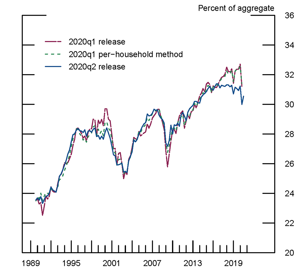
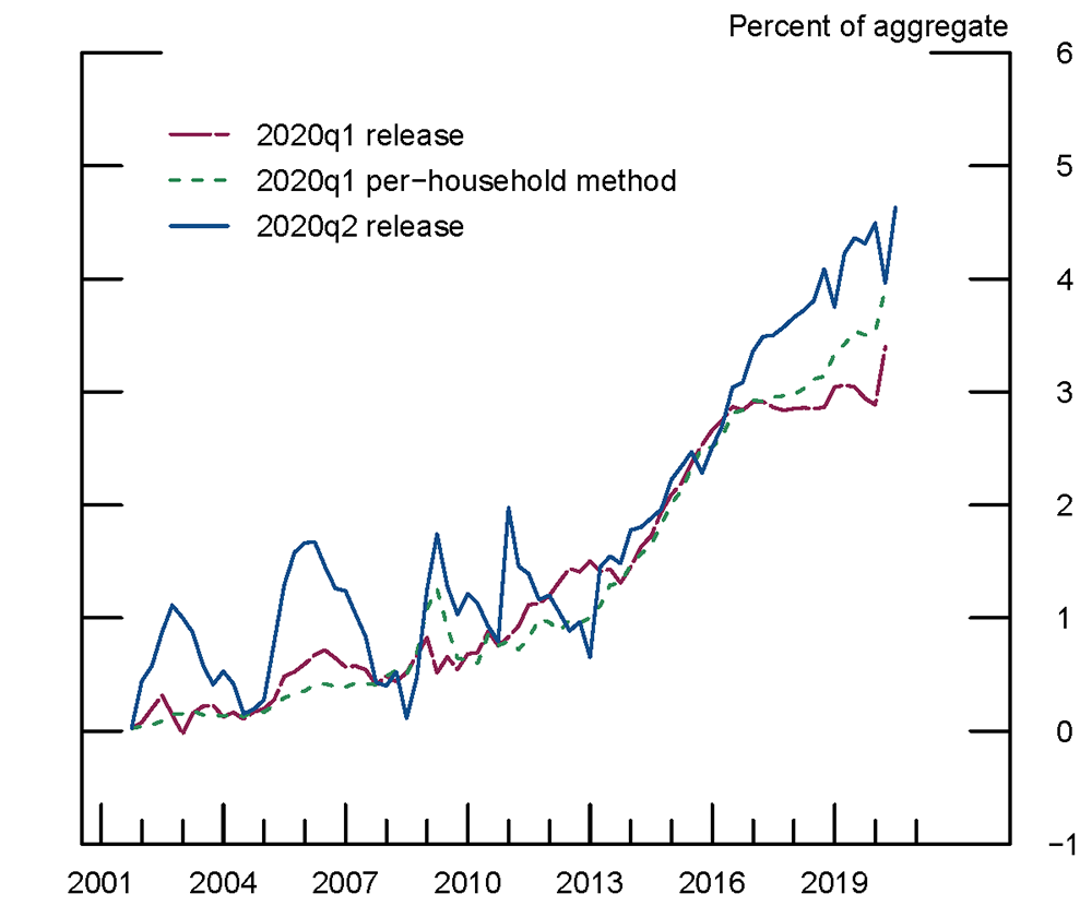
Figure 1 compares the wealth share of the top 1 percent of the wealth distribution ("Top 1") in our new 2020q2 DFA release with our previous release for 2020q1. Looking at the big-picture effects, the new release shows a small decline in the Top 1 percent share since 2016. The 2019 SCF reveals that the Top 1 share did not rise between 2016 and 2019—in fact, it came in nearly one percentage point lower in the 2019 SCF than in the 2016 SCF (Bricker, Goodman, Moore, and Volz, 2020). Thus, the difference between the 2020q1 and 2020q2 DFA releases for the Top 1 share since 2016 primarily reflects the 2019 SCF data, not the methodological updates. The slow decline in Top 1 share, compared with the increase predicted in 2020q1, is accounted for by this group's falling share of time deposits, pensions, and equity in noncorporate business, as well as a slightly slower-than-projected increase in their share of corporate equities and mutual funds. Strong growth in housing wealth for the bottom half of the wealth distribution also contributed to the fall in the Top 1 share, but this change was largely anticipated by the projections in the 2020q1 DFA and thus did not result in significant revisions when the 2019 SCF was incorporated.
The quarters since the 2019 SCF have been characterized by economic fluctuation and market volatility. The wealth share of the Top 1 increased at the end of 2019 with the strong equity market performance in the fourth quarter, but then fell sharply in 2020q1 as the onset of the COVID-19 pandemic caused large market declines. Inequality increased again in 2020q2 as markets began to recover, but the wealth share of the Top 1 remains 0.4 percentage points lower than at the 2019 SCF as the savings generated by the pandemic-related reduction in spending and generous income support from the CARES Act have been spread throughout the distribution, and equity markets had not yet returned to pre-pandemic highs.
Since the Top 1 wealth share did not increase in the SCF despite generally strong readings from our indicator series between the 2016 and 2019 SCFs, the updated temporal disaggregation models for the Top 1 share are modestly less pro-cyclical throughout the DFA history. As shown in Figure 1, the effects of this change are apparent during the tech bubble of the late 1990s, for which the new model shows a smaller rise in the Top 1 share, and during the Great Recession, for which the new model shows a smaller decline in the Top 1 share.
Figure 1 also shows how our shift to estimating models on a per-household basis contributes to the reduction in the pro-cyclicality of the Top 1 wealth share. In particular, the 2020q1 – per-household method series shows that had the 2020q1 release employed temporal disaggregation models that were estimated on a per-household basis, the peak in the tech bubble and trough in the Great Recession would have both been diminished.5 The reduced cyclicality for the Top 1 share from this modelling change is driven by corporate equity and mutual funds. Under the method employed in previous releases, the estimated coefficient on household count was negative for two of the wealth groups. After removing household count as an indicator and switching to per-household estimation, the coefficients on the Financial Accounts corporate equities and mutual funds series for the four wealth groups moved closer to each other, and, thus, the shares of this asset category, including the Top 1 share, no longer change as quickly when the market turns.
By definition, the share of wealth lost by one group is gained by other groups. Relative to prior releases, the DFA wealth share lost by the Top 1 percent as a result of incorporating the 2019 SCF is largely gained by the next 9 percent, leaving the shares of the bottom 90 percent of the wealth distribution mostly unchanged. In contrast, the new estimation methodology slightly reduces the counter-cyclicality of both the Next 9 (families between the 90th and 99th percentiles) and Next 40 (families between the 50th and 90th percentiles) wealth shares.
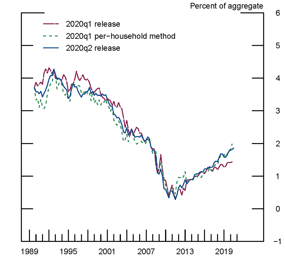
The 2019 SCF also reveals that, compared to prior DFA releases, the share of wealth held by the bottom 50 percent of the wealth distribution grew more quickly since 2016. As shown in Figure 2, per-household estimation more accurately predicts this increase, with much of the difference stemming from the model for home mortgages.
Other Wealth Splits
Incorporating the 2019 SCF and applying our updated methodology also generates revisions to the other wealth splits (by income, age, generation, education, and race) in the DFAs. In general, these revisions are modest, with the most notable changes typically occurring in the post-2016q3 quarters for which the 2019 SCF gives us substantial new information.
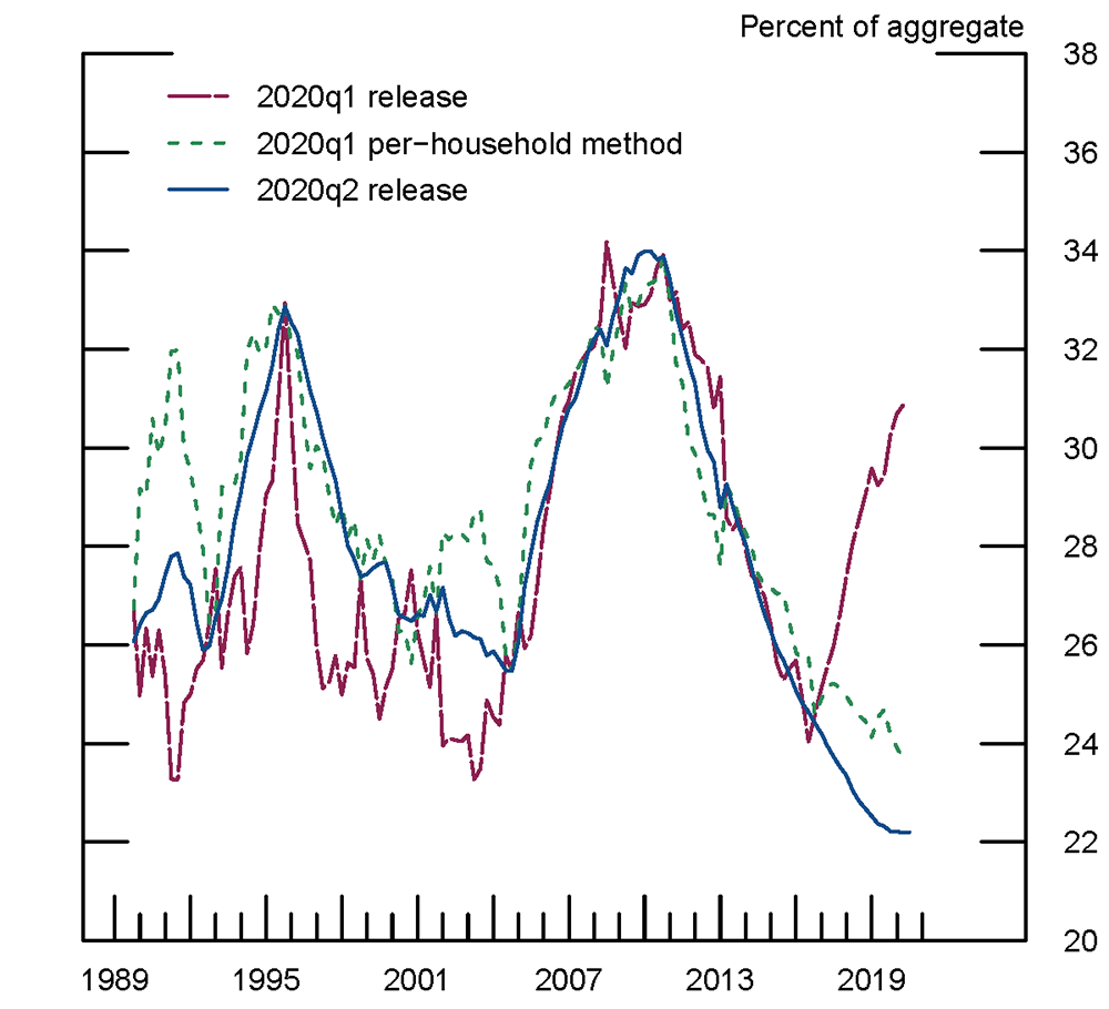
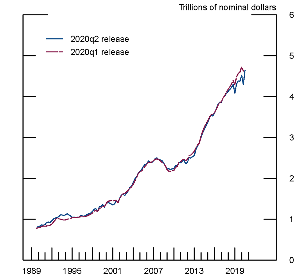
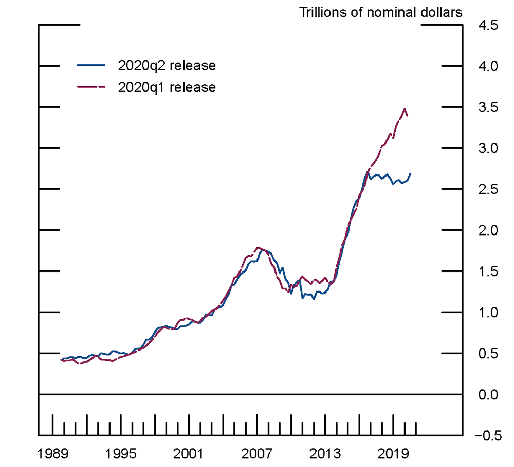
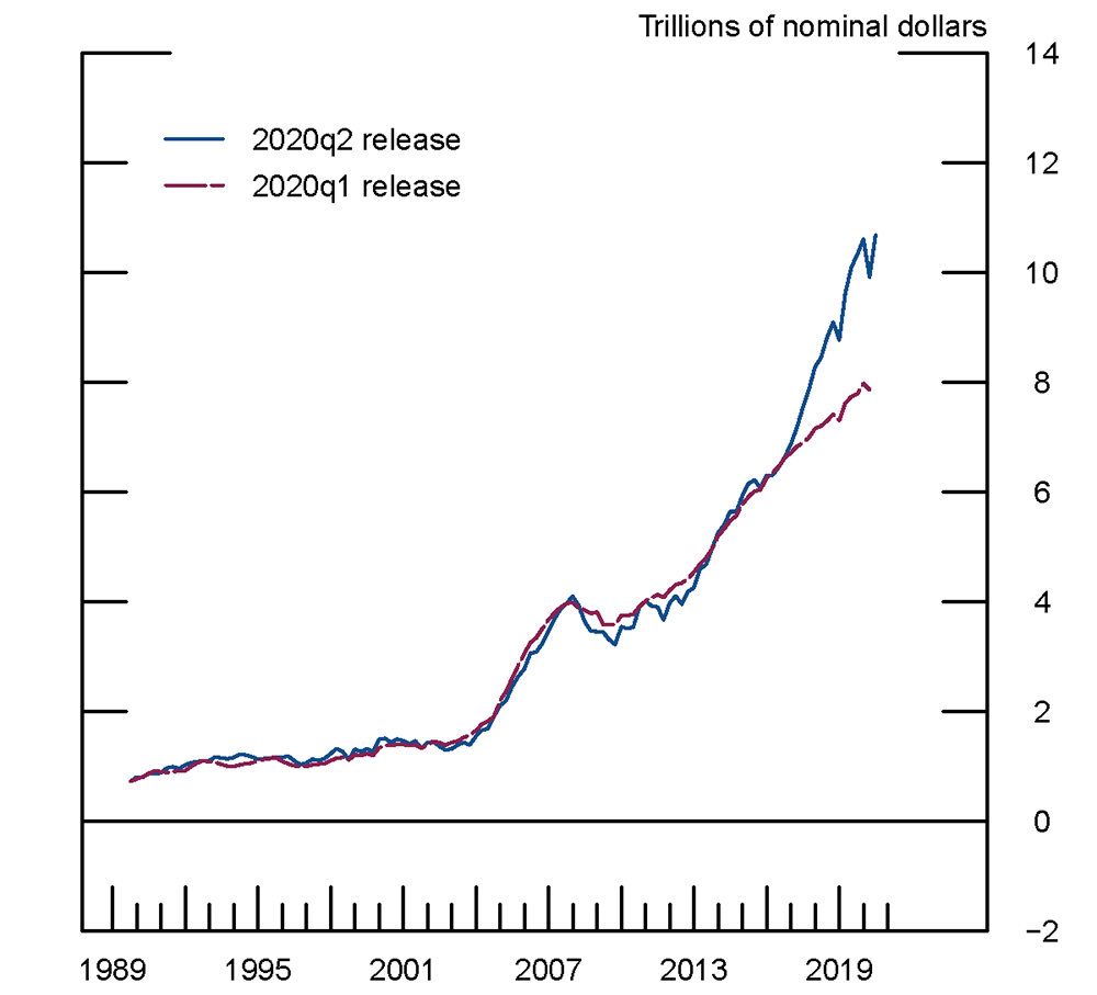
For instance, the 2019 SCF provides new insight on the distribution of wealth by race. 6 As shown in Figure 3, white and Black DFA net worth since 2016 came in close to the levels projected in the 2020q1 DFA. By contrast, Hispanic net worth came in lower than projected, while "other" net worth came in higher. The slower-than-projected growth of Hispanic net worth between 2016 and 2019 is driven by a decline in corporate equity and mutual fund holdings in the 2019 SCF for this group, after a spike in 2016, back to a level similar to the 2010 and 2013 SCFs.7
Figure 3a-d
The updated methodology and the incorporation of the 2019 SCF both contribute to the revisions in the wealth-by-generation DFA estimates. Because the evolution of the generation sizes is a first-order driver of their wealth shares, using per-household estimation more accurately models the dynamics of wealth for each generation. Indeed, we do find that the per-household models generally perform better for the generational wealth splits. For example, Figure 4 shows that they better predict the increase in millennial wealth since 2016. Much of the remaining difference stems from the fact that the 2019 SCF includes more Millennial households than was projected in the 2020q1 DFA. Similarly, updates to the number of households explains a large amount of the updates to the wealth shares of the other generations.
Note: Observations of Millennials are available beginning with the 2001 SCF.
Conclusion
The 2020q2 release of the DFAs integrates two methodological improvements with updated wealth information from the just-released 2019 SCF. Among other changes, the new DFA release shows that the share of wealth held by the top 1 percent of the wealth distribution was flat or decreasing in the years since 2016, consistent with the 2019 SCF. In the quarters since, wealth inequality has fluctuated with the effects of the COVID-19 pandemic and the government response.
References
Fernandez, R. B. (1981). A methodological note on the estimation of time series. The Review of Economics and Statistics, 63(3):471{476.
Chow, G. C. and Lin, A. (1971). Best linear unbiased interpolation, distribution, and extrapolation of time series by related series. The Review of Economics and Statistics, 53(4):372{375.
Batty, Michael, Jesse Bricker, Joseph Briggs, Sarah Friedman, Danielle Nemschoff, Eric Nielsen, Kamila Sommer, and Alice Henriques Volz. "The Distributional Financial Accounts of the United States." In Measuring and Understanding the Distribution and Intra/Inter-Generational Mobility of Income and Wealth. University of Chicago Press, 2020.
Bricker, Jesse, Sarena Goodman, Kevin Moore and Alice Henriques Volz. "Wealth and Income Concentration in the SCF: 1989-2019." FEDS Notes. Washington: Board of Governors of the Federal Reserve System, September 28, 2020, https://doi.org/10.17016/2380-7172.2795.
1. https://www.federalreserve.gov/econres/scfindex.htm Return to text
2. For example, the inclusion of the 2019 SCF data alter the estimated empirical relationships between different groups' holdings of equity in noncorporate business (e.g., small businesses) and the S&P 500 index. As a result, we have changed the indicator series we use to model the evolution of equity in noncorporate businesses from the S&P 500 index to measures of residential and commercial real-estate holdings. Return to text
3. The count of households for each group are taken directly from the SCF in quarters that coincide with an SCF release. Between SCF surveys, we estimate the count of households for each group using a cubic spline. Return to text
4. The few cases occurred among groups with small sample sizes in the SCF. Return to text
5. In this estimation, we do not incorporate the 2019 SCF or the 2020q2 release of the Financial Accounts. Switching to the Fernandez method from the Chow-Lin method had virtually no further effect on the time series of the Top 1 share. Return to text
6. Race is reported by the respondent and refers to the survey respondent rather than the household composition. It is recorded as one of four mutually exclusive groups: white non-Hispanic, Black non-Hispanic, Hispanic, and "other," which includes respondents not covered by the first three groups (including respondents who identify as multi-racial). Return to text
7. Looking more closely, the high value for Hispanic corporate equity and mutual fund holdings in the 2016 SCF is driven by a relatively small number of households with high direct stock holdings. Return to text
Batty, Michael, Jesse Bricker, Ella Deeken, Sarah Friedman, Eric Nielsen, Kamila Sommer, Sarah Reber, and Alice Volz (2020). "Updating the Distributional Financial Accounts," FEDS Notes. Washington: Board of Governors of the Federal Reserve System, November 09, 2020, https://doi.org/10.17016/2380-7172.2810.
Disclaimer: FEDS Notes are articles in which Board staff offer their own views and present analysis on a range of topics in economics and finance. These articles are shorter and less technically oriented than FEDS Working Papers and IFDP papers.